AFT Blog

Well, if the answer is "more than one", then you are probably struggling to deal with way more model files than you need to be.  With all AFT products, the Scenario Manager is an incredibly powerful feature that allows one to model several different cases within a single model file. This includes different operating conditions, multiple pump configurations, different piping, system expansions, hot days, cold days, insulation, fouling and pipe scaling, etc. The list of different cases that can be modeled is essentially endless! So, I have said it once, and I will say it again...The Scenario Manager is one of...

Well that depends on how optimistic you are, but either way you can model partially full pipes with AFT Impulse! This means partially full along the axial direction, as opposed to partially full along the radial direction. This function only works for pipes that have a slope, and when the pipe is partially full it drains from the end with the higher elevation. Pipes which contain vacuum breaker valves, exit valves, spray discharges, or assigned pressures at the outlet can drain or fill during the transient. This draining or filling is limited to the specified pipe. AFT Impulse will not model...

When dealing with a compressible gas system, heat transfer and thermal effects are very important to account for.  When a gas is flowing down a pipeline, it will cool down as the gas expands due to the frictional pressure drop.  Many would say that adiabatic or isothermal conditions will bracket the potential flow rates that are possible for a constant pressure drop in a pipe.  However, this is not the case.  If a gas is cooled or heated as it flows down the pipeline, the flow rates that can result for a given pressure drop can actually be outside the “bounds”...

In AFT Arrow, there are three types of fluids that can be modeled:  AFT Standard, ASME Steam, and Chempak.  The focus of this article will be on how to use the Chempak Database with AFT Arrow in order to perform dynamic mixing calculations.  But first, I would like to briefly introduce each of the three types of fluids that can be modeled in AFT Arrow. The gases in the AFT Standard fluid list are included with the standard AFT Arrow software.  Various equation of state models are available including Ideal Gas, Constant Z, Three Parameter, and Redlich-Kwong.  There are also multiple...

Many engineers are familiar with gas accumulators and their ability to aid in surge suppression modeled in AFT Impulse, but what about liquid accumulators? Liquid accumulators are different from gas accumulators in that they are assumed to be liquid full and do not have any gas that can compress and expand in order to dampen pressure spikes caused by water hammer.  Liquid accumulators change the system response to pressure spikes, but they operate differently than gas accumulators. There are only three required input parameters for liquid accumulators; Elevation, Elasticity, and Initial Volume. Figure 1: Liquid Accumulator Properties Window Initial Volume is...

It is possible to model the shell side and tube side of a heat exchanger in AFT Fathom and AFT Arrow where the “hot fluid and cold fluid” circuits can also be included for both sides of a heat exchanger in a single model file!  This can be accomplished by creating a "thermal link" between two heat exchangers and using the “Heat Transfer with Energy Balance (Multiple Fluids)” option in the System Properties window. 

As shown in Figure 1 below, there are two separate systems modeled on the same Workspace.  The left side of the system is an auxiliary cooling water loop while the right side system is the hot oil circulation loop.  The two heat exchanger junctions that are highlighted in the red box, J8 and J18, represent the tube side and shell side of a single heat exchanger.  The cooling water circuit is on the tube side of the heat exchanger and the hot oil loop is on the shell side of the same heat exchanger.  These heat exchanger junctions are “thermally linked” together, as they represent the same physical heat exchanger.  Therefore, their resulting heat rates will be the same, but opposite in sign.

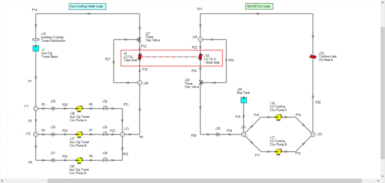
An important requirement to keep in mind that will allow the modeling of two sides of a heat exchanger with the “thermal linking” feature is that both fluids on each side of the heat exchanger must remain in fully liquid phase for AFT Fathom (or fully gas phase for AFT Arrow).  Therefore, there cannot be any phase change in either fluid circuit or through the heat exchanger itself.

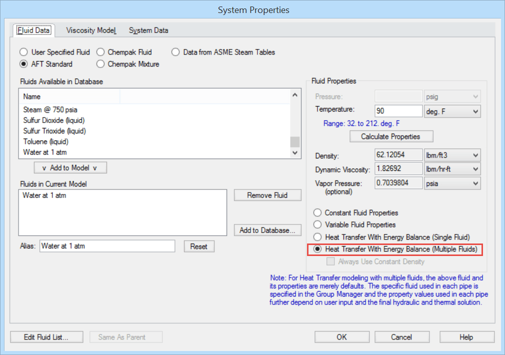
First step is to build a model of the system and include both cooling water and hot oil loops.  After all the pipes and junctions are laid out on the Workspace (but not defined), open up the System Properties window and choose the "Heat Transfer with Energy Balance (Multiple Fluids)" option as displayed in Figure 2.  A single “default” fluid must be selected and defined.  The individual fluids used in each loop will be defined soon.

Next, the pipes and junctions can be defined with their various thermal models and characteristics (except for the two heat exchanger junctions that will need to be modeled as two sides of one heat exchanger. This will be specified later).

In order to use the "Multiple Fluids" option in System Properties so that two sides of a heat exchanger can be thermally linked, "Fluid Groups" must be created.  Before fluids can be assigned to specific “Fluid Groups”, separate groups of all the pipes and junctions in each individual circuit need to be created first.

As shown in Figure 3, select all the pipes and junctions that make up one of the circuits, such as the cooling water loop.  Then from the Edit menu, click "Groups", then "Create", and give that group of pipes and junctions that are selected, a name.

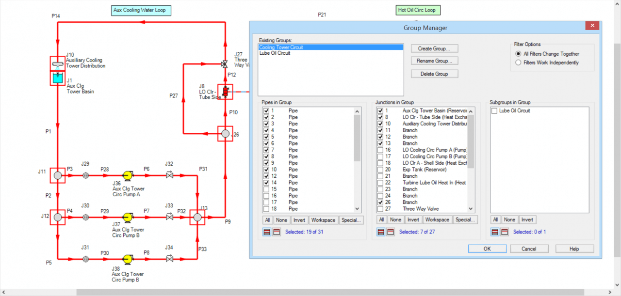
Then, select the pipes and junctions that make up the hot oil side. With those objects selected, click "Edit", then "Groups", then "Create" and give the hot oil loop a name.

After two separate groups for each loop have been created, the specific fluids that will be used for each group can now be defined.  Click "Edit", then "Groups", then "Fluids".  Check both boxes so that both fluid groups can be used.

For the cooling water circuit, click the box with the little dots in the "Fluid" column, then specify the fluid properties, like that in Figure 4.  Any of the fluid options are available, except for "User Specified Fluid" (because the "User Specified Fluid" option does not model heat transfer).

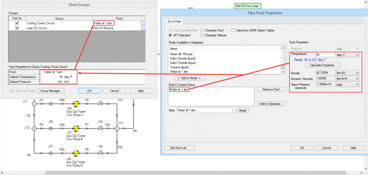
Then, specify the fluid properties for the hot oil loop by clicking on its box with the little dots.

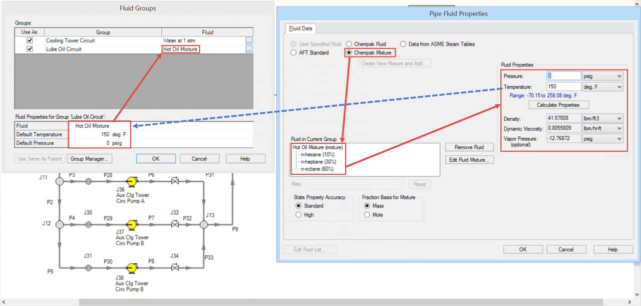
After a particular fluid has been chosen for each fluid group, click OK.

Now, the two heat exchangers can be "thermally linked" together.

Open one heat exchanger, and on the Thermal Data tab, specify one of the Effectiveness-NTU thermal models, then check the box to "Link to Heat Exchanger", and select the other heat exchanger from the drop-down menu that you want to link to. Then specify the required parameters.  Figure 6 illustrates how to thermally link the cooling water loop tube side with a “Counter-Flow” thermal model and it will link to the Hot Oil Loop heat exchanger.

AFT Arrow solves all of the fundamental controlling equations governing gas dynamics. For more information about which fundamental thermodynamic equations are solved in AFT Arrow, here is an excellent article that discusses gas flow calculations in detail.   The "stack effect" is simply one aspect of these equations, and is accounted for by the user input and boundary conditions. Ultimately, flow is driven by pressure difference. The higher you raise a chimney, the lower the atmospheric density and pressure at the discharge. In order to accurately model the "stack effect", the system boundary conditions must be modeled accurately.  As the discharge...