AFT Blog
The primary way to view results when using Impulse is through graphical data. With the release of AFT Impulse 6, the power of the graphing features has been greatly increased. With this enhanced capability comes additional complexity. It is a kin to the power and complexity of in-dash radio consoles in modern cars compared to the old stereo in my old Ford Pinto. To help users navigate the new capabilities of this powerful graphing tool, we have developed a ‘Graph Guide’ which points out the steps to accomplish many of the common tasks in creating, modifying and keeping graphs. The Graph...
You’ve built your AFT Fathom or AFT Arrow model, defined all pipes and junctions, specified your fluid properties and defined your pressure boundary conditions. But for some reason, your predicted flows are still not matching measured data. AFT Fathom or AFT Arrow is properly solving the fundamental equations, but it is likely that something is off in the inputted data. In many cases, this is the pipe’s resistance. Many factors can alter a pipe’s resistance, but the two primary reasons resistance may be incorrect is (1) corrosion of the pipe over time, which increases a pipe’s absolute roughness and (2) the buildup of residue on the walls of the pipeline, known as scaling, which decreases a pipe’s inner diameter. This decrease in diameter is very important and will increase a pipe’s resistance dramatically. Now you have a dilemma. You can’t cut open your pipe to see how much scaling there is or how much your pipe has corroded. What is the condition of your pipe? Using AFT Fathom GSC or AFT Arrow GSC, you can find out!
Amongst the vast multitude of superbly efficient features within AFT Software, the customization and Database capabilities are certainly of significant importance. If you are not familiar with how to use the Databases within our software to manage your customized information, then getting familiar should be a top priority for what you learn how to do next in our software. Making effective use of Databases will save you and your team of AFT users incredible amounts of time! The vast amounts of data that you can customize within our software includes: Components (junctions)Fluid propertiesPipe materialsPipe insulationFittings & Losses (that get lumped into...
Often times when building larger network models, you may not be sure what the direction of the flow will be and running the model is the only way to determine the flow direction. In the below AFT Arrow model it might be hard to determine what way the flow convention is in some of the loops. After running this model there are cautions stating that flow is negative through junctions that may have loss factors that are dependent upon direction. What is the easiest way to fix this? You could compare your results, remember or make a table of what pipes...
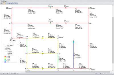
Each AFT software product employs five Primary Window tabs in which you would build, define, and analyze the model of your system. Of these, the Visual Report window is incredibly useful in that you are able to overlay your model input or output parameters directly on top of the graphical layout of the system itself. This is an excellent feature to use when you want to provide the bottom line results to clients and colleagues at a high level (or a detailed level). Figure 1 is an example of what the Visual Report for a particular system might look like. As...
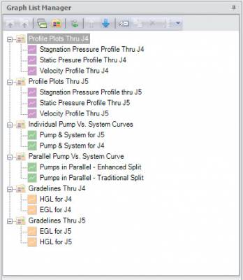
AFT software products have had powerful graphing capabilities for a very long time. Many types of graphs can be created with AFT products such as pump vs. system curves, profile plots along a flow path, gradelines and elevation profiles, transient plots (with AFT Impulse or the AFT Fathom XTS module), slurry system curves (with AFT Fathom SSL or AFT Impulse SSL modules), and selected solutions that allow you to plot various output parameters for desired pipes. All of these graphing capabilities are incredibly important to engineers as they analyze the hydraulic behavior of their system. The ability to customize the graphs...
One of the newest features of AFT Fathom 9 that will add a lot more efficiency to analyzing your results is the new Design Alert Manager! In addition to the new Design Alert Manager, it is also possible to add general Design Alerts for junctions such as inlet or outlet pressure, or perhaps the pressure loss across a junction. In previous versions of our software, it would be possible to create different Design Alerts for pipes where you could specify a minimum or maximum value for a particular output parameter such as a maximum pressure limit, minimum flow rate, maximum velocity,...


