


AFT Blog
Welcome to the Applied Flow Technology Blog where you will find the latest news and training on how to use AFT Fathom, AFT Arrow, AFT Impulse, AFT xStream and other AFT software products.
14 minutes reading time
(2798 words)
Featured
Know Your Pump & System Curves - Part 3

In the final "Know Your Pump & System Curves" blog series, I am going to discuss the complexities behind pump vs. system curves for systems with pumps in series and parallel configurations. Multiple pumps in series configurations are relatively straight-forward and will be discussed briefly. Operating pumps in parallel configuration involve a few complexities that can be confusing. Therefore, this article will focus primarily with operating pumps in parallel configurations.
If you have not had a chance to read the previous blogs, please be sure to do so to get a better pre-requisite understanding of pump and system curves and how AFT Fathom generates them. Here is where they can be found.
Know Your Pump & System Curves – Part 1
Know Your Pump & System Curves – Part 2A
Know Your Pump & System Curves – Part 2B
The pump and system curve concept for multiple pumps in series or parallel that has not been discussed in the previous blogs is that of a "composite" pump curve and a "composite" system curve. In series and parallel configuration, it is not typical to generate the pump and system curves for a specific pump individually. Instead, composite curves represent the combined performance and resistance for the pumps acting together.
Let's start the discussion with multiple pumps in series configuration. In Figure 1 below, there are two pumps in series, separated by 3,000 feet of piping with an overall system elevation change of 200 feet. As you can see, the pumps are different with different pump curves. Both have 9-inch impellers, but one operates at 3,179 rpm while the other operates at 3,550 rpm.
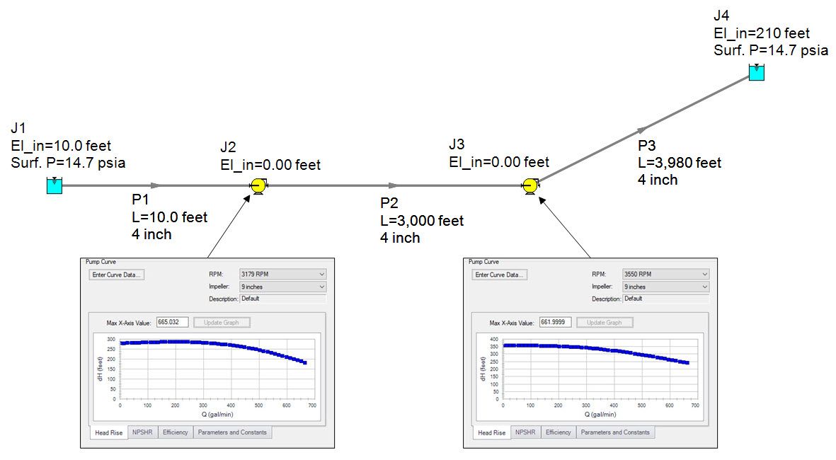
Figure 1 - Operating to dissimilar pumps in series configuration.
At a given flow rate, the head rise from each pump's individual curve is added together to obtain the composite pump curve for pumps in series. Figure 2 plots many pump and system curves together. First, concentrate on the different individual pump curves for J2 and J3. AFT Fathom easily creates the composite pump curve with the click of a button. To verify the composite curve, I used the AFT Fathom eXtended Time Simulation (XTS) module similarly to the previous blogs to determine a common flow rate through each pump at a given time step to easily calculate the pump head added across each pump. Then I manually added the total head for pumps J2 and J3 at a given flow to obtain a manual composite pump head. As you can see, the manual composite curve I calculated by adding the pump heads at each flow matches exactly the composite curve calculated by AFT Fathom.
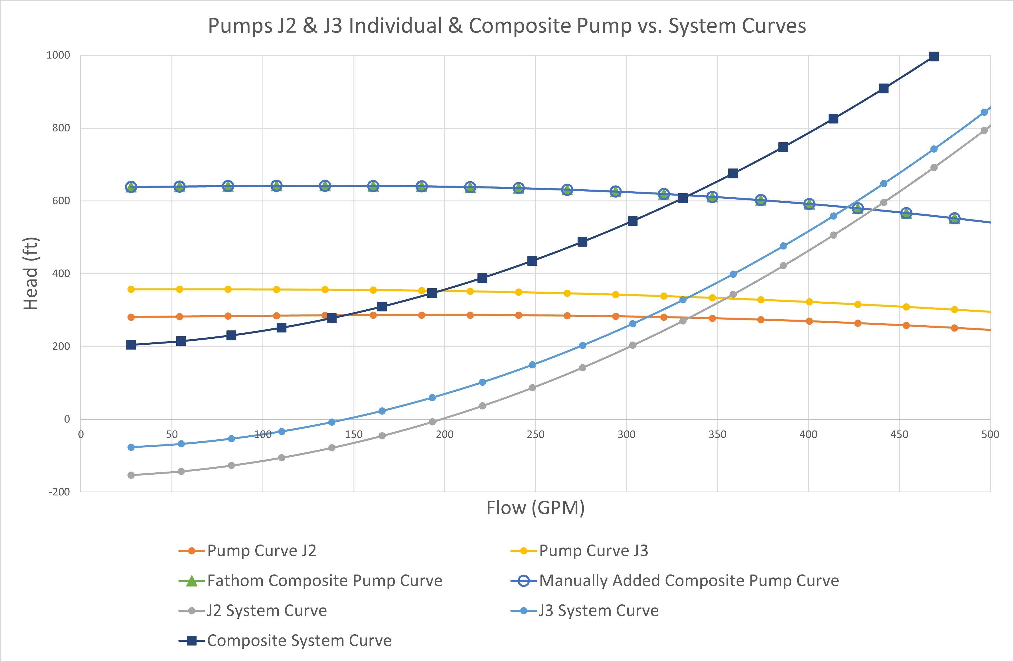
Figure 2 - Pump & system curves plotted for pumps in series configuration from Figure 1. Individual pump curves are plotted. Composite pump curve is equal to the individual pump curves added together with respect to pump head at a given flow.
Now, let's focus on the system curve side of things for the plots in Figure 2. There is a system curve plotted for pump J2 as well as for J3. The way these two individual system curves are obtained is by setting one pump to a pseudo-fixed flow pump and running the model in the background over a range of flows and calculating the required pump head. This process generates the system curve for that specific pump. Keep in mind that during this process, the other pump is simply operating on its curve. Just like how AFT Fathom generates system curves as discussed in the previous blogs in this series.
The composite system curve is slightly different. We only need to use one of the pumps in series to generate the composite system curve. One of the pumps is set to the pseudo-fixed flow model while the other pump takes on a special condition called "Pump Off with Flow Through". This special condition basically ignores the pump for modeling purposes and the pump acts like a Branch junction. Therefore, when the system curve is generated for just one of the pumps and the head is calculated at each flow rate, this head requirement does represent the entire system resistance and elevation change seen by that specific pump.
On my own, I tested this by running two scenarios. In one scenario, I generated a system curve for pump J2 while setting pump J3's Special Condition to "Pump Off with Flow Through". The other scenario, I switched the operation so that pump J2 had the Special Condition applied while the system curve was generated for pump J3. When I generated the system curves manually for J2 and J3 individually in this manner, the system curves exactly matched the composite system curve for both pumps in series.
Overall, obtaining a composite pump curve and composite system curve for pumps operating in series in AFT Fathom is not too complicated. Well, AFT Fathom does it all for you! But now it should be better understood what AFT Fathom is doing in the background to generate these curves.
Onto the next part of the discussion regarding multiple pumps operating in parallel. The rest of the article will cover the following points.
- Identical pumps with identical curves operating in parallel to add flow
- How much flow that pumps in parallel add depends on shape of the system curve
- How composite pump and system curves are generated
- Traditional Method vs. Enhanced Method
- Impact of operating dissimilar pumps in parallel
- Impact of operating identical pumps with identical pump curves in parallel with dissimilar piping
- This effect is very very small
The operating point for the simple pipeline in Figure 3 below is 500 GPM and the pump adds 245 feet of Total Dynamic Head (TDH). At the operating point, the pump operates at its Best Efficiency Point (BEP) because the pump was properly sized and selected for this pipeline.
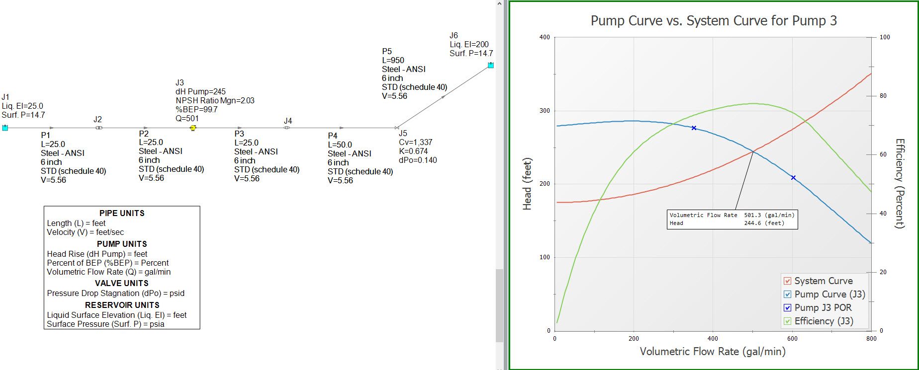
Figure 3 - Simple pipeline with a single pump operating to establish base case for operating multiple pumps in parallel with this system.
To deliver more flow through a system, a potential solution is to add a second pump in parallel. The traditional thought is that the pump curves are additive in terms of flow like in Figure 4. But how much more flow will they add? Let's say there is a new flow demand in our pipeline from Figure 3 for 50% more flow of 750 GPM. Figure 5 A represents the attempt to add an identical pump in a parallel configuration with symmetrical piping.
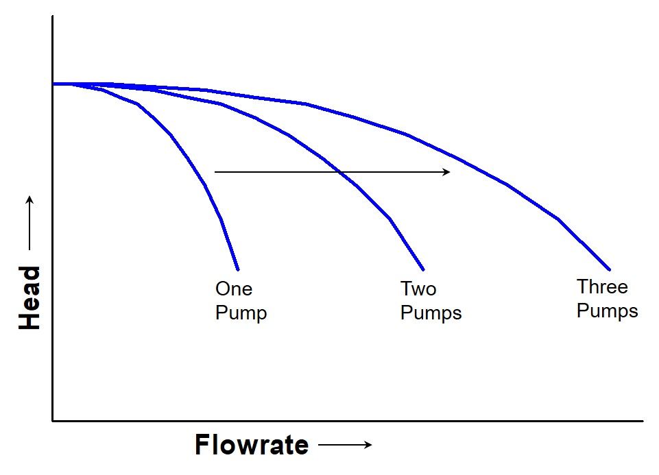
Figure 4 - Conceptual operation of multiple pumps in parallel with the goal to increase flow. Pump curves add to the right with respect to flow at a given pump head.
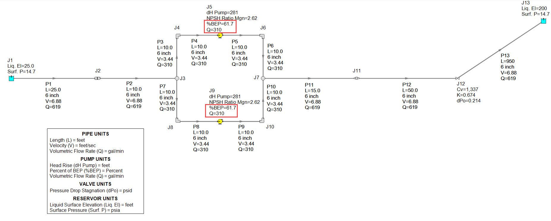
Figure 5A - Models two pumps in parallel with symmetrical piping.

Figure 5B - System models three pumps in parallel with slightly non-symmetrical piping.
As you can see, the increase in flow through the pipeline is far less than what we were hoping for. We only got about 24% more flow with a second pump in parallel as in Figure 5 A and we were hoping for 50% more flow. Clearly, the flow did not double, which is sometimes expected. Also, be sure to notice that the pumps are now operating much further away from their BEP. Figure 5 B models three identical pumps in parallel with non-symmetrical piping which only generates 3% more flow, increasing from 619 GPM with two parallel pumps to 634 GPM with three parallel pumps! Very quickly we approach a point of diminishing return where adding more pumps does not generate that much more flow.
One primary reason we do not get much more additional flow is simply because the water pipeline system and pumps are not sized for the additional flow capacity. To get a significant increase in the system, the system and design itself needs to change. The other reason can be explained with the shape of the system curve itself.
Figure 6 A & B demonstrate the quantitative amount of additional flow for a frictionally dominated system (Figure 6A) compared to a static dominated system (Figure 6B). Frictionally dominated systems are cases where most of the system resistance a pump needs to overcome is frictional resistance is significant. The elevation changes a pump must overcome is small in comparison to frictional losses. Closed systems are often frictionally dominated systems. In frictionally dominated systems, system curves will typically be much steeper and the additional flow from additional pumps will be small. Static dominated systems are when the primary resistance a pump must overcome is elevation changes. The frictional resistance is small in comparison. Figure 6B represents a static dominated system and as you can see, this is a case where additional pumps in parallel can deliver additional flow. But there will still be a point of diminishing return where each additional pump generates less flow.
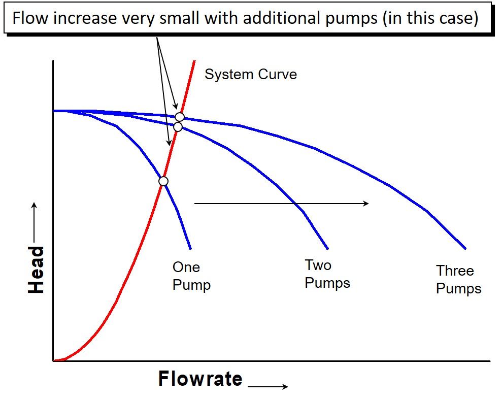
Figure 6A - Steep system curve for frictionally dominated system where additional pumps do not add much increase in flow.
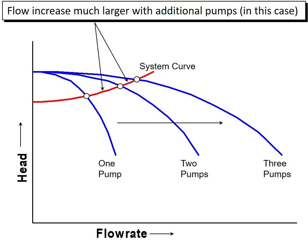
Figure 6B - Flatter system curve for static dominated system in bottom image where multiple pumps in parallel can help increase in system flow.
Figure 7 shows the pump and system curves plotted together for our pipeline in Figure 3 with one pump operating, Figure 5A with two pumps operating in parallel, and Figure 5B with three pumps operating in parallel. The pump curves are added together for operating two and three pumps in parallel. Although the piping at the pumps is slightly different for each configuration from using one to three pumps, the system curve is essentially the same. Although the system curve does not appear to be very steep, you can see that the frictional losses become more significant when attempting to deliver more flow through the system with additional pumps.
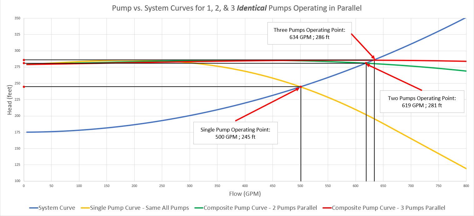
Figure 7 - Pump & system curve plotted for systems in Figure 3, 5A, and 5B. Goal was to increase system flow by 50% with a second pump, where adding a second pump in parallel only increased flow by 24%. A third pump in parallel only increases flow by an additional 3%.
Table 1 provides a summary of the operating points for each configuration. Notice how much further away from BEP each pump operates with two or three pumps in parallel. More flow at the expense of reliability is probably not worth it.
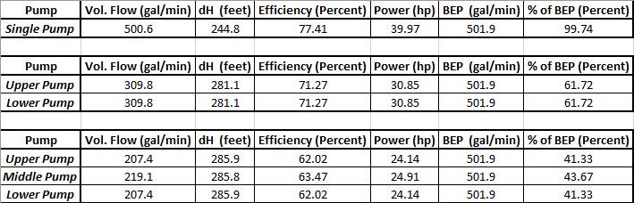
Table 1 - Pump operating conditions for systems in Figure 3 (1 pump), 5A (2 pumps in parallel), and 5B (3 pumps in parallel). Note the dramatic decrease in proximity for each pump’s BEP for each parallel configuration.
Consider the operating points from Table 1 for two or three pumps in parallel. It is apparent that the composite operating point where the composite pump and system curves intersect is the total flow through each pump added together while the pump head is the average of each of the individual pumps. However, this is NOT by design and the composite operating point only happens to be the case because the pumps and their curves are identical, and that this system is very symmetrical.
There are two methods that AFT Fathom uses to generate the composite pump & system curves for parallel pump operation. They are referred to as the "Traditional Method" and "Enhanced Method".
The "Traditional Method" assumes an equal flow split across all pumps at all flow rates during the curve generation process. When plotting the composite pump curve, AFT Fathom takes the total composite flow, splits it evenly across each pump, calculates the pump head for each pump, and then averages the pump heads together. Generating the composite system curve is quite similar with splitting the total composite flow equally across the pumps, calculates the pump heads required at each pump's flow, and then averages those pump heads together.
The traditional method is accurate and works well when the pumps operating in parallel are identical to the manufacturer, model, pump curve, etc. as well as when the pump piping through each parallel path is symmetrical.
The way the "Enhanced Method" works is that the pump curves are simply added to the right with respect to flow rate to generate the composite pump curve. There is no attempt to split flow across the pumps. When the pump curves are added together like this, there is a unique value for the pump head at each flow rate. This can lead to an odd-looking composite pump curve for non-identical pumps operating in parallel.
Composite system curves generated using the "Enhanced Method" will determine the flow split through each parallel pump at the operating point. Then, assuming the flow split remains the same across the entire range of flows, the same flow split ratio is apportioned to each pump accordingly when calculating the required pump head for each pump. Those pump heads are then averaged together.
If the pumps are identical and the suction and discharge piping is symmetrical, then the composite pump curves and system curves will be the same when using either the Traditional or Enhanced methods.
A case when the composite pump vs. system curves can be different between the Traditional and Enhanced methods is when dissimilar pumps are operating in parallel. This is well illustrated with the AFT Fathom Example Help File model called the "Hot Water System", as shown in Figure 8. The problem statement and goals of that example are slightly different than the purpose for this blog series. I modified the system by setting the Special Condition of the Control Valves to "Fully Open – No Control" and I changed the pump curves so that the system is operating three different pumps in parallel.
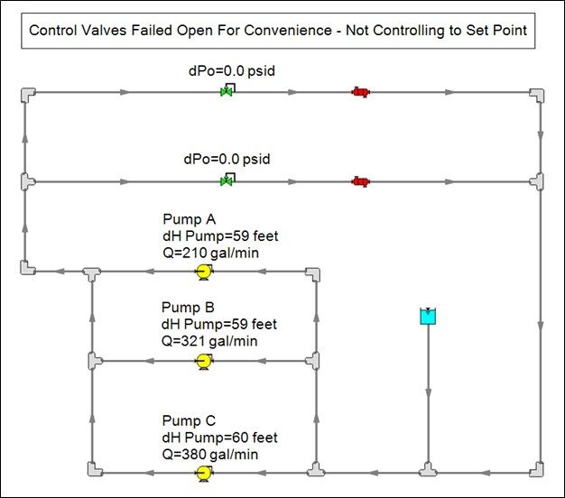
Figure 8 - “Hot Water System” example for operating three dissimilar pumps with non-symmetrical piping in parallel. Flow Control Valves set to “Fully Open – No Control” Special Condition for modeling convenience.
Plotted in Figure 9 is each individual pump curves for Pump A, Pump B, and Pump C. Also plotted is the composite pump curve with the Traditional Method and the composite pump curve with the Enhanced Method. It turns out that the Composite System Curve is the same for the Enhanced and Traditional Methods. As you notice, the composite pump curve with the Enhanced Method takes on an odd shape and this is simply the artifact of operating dissimilar pumps in parallel where the curves are added to the right with respect to flow rate. When examining the plot closely, you will see that the Enhanced Composite Pump Curve crosses the Composite System Curve at the total flow rate of each pump from Figure 8 and the average head across each pump.
The Composite Pump Curve with the Traditional Method does NOT cross the Composite System curve at the total flow rate for each pump. This is where some ambiguity lies regarding generating composite pump and system curves for operating dissimilar pumps in parallel.
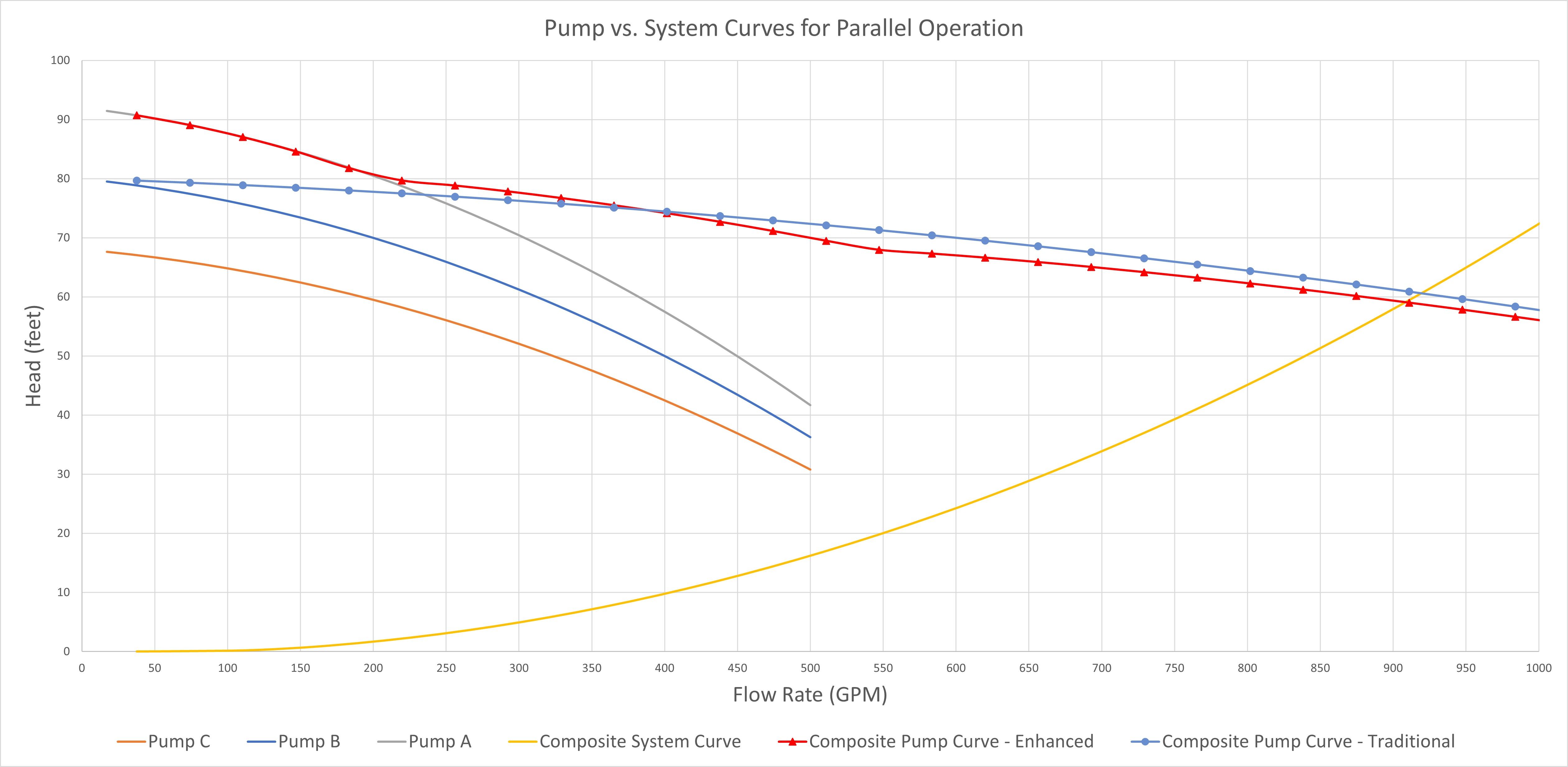
Figure 9 - Pump and system curves plotted for operating three dissimilar pumps in parallel with non-symmetrical piping in Figure 8. Note the differences where the composite pump curves cross the composite system curves with respect to Enhanced vs. Traditional Methods for parallel curve generation.
Overall, operating dissimilar pumps in parallel or pumps in parallel with non-symmetrical piping should be avoided. This can lead to some ambiguity when there are multiple ways the composite curves can be generated and how sometimes the composite curves may not cross at the operating point. But more importantly, the pumps would tend to "compete" with each other for a dominating flow rate. This is an issue because it can cause one of the pumps to operate closer to its BEP than the other(s). This can lead to reliability problems for the pumps that operate further away from BEP as they experience various issues such as those discussed in this blog here. The pumps will not wear evenly and ultimately will lead to increased repair costs, more down time, loss profits, production losses, etc.
This concludes this article regarding pump and system interaction for pumps in series and parallel configuration as well as the "Know Your Pump & System Curve" blog series. Hopefully, this helps clear up the various nuances that can be sometimes confusing for generating pump and system curves. Thank you very much for reading!
Comments