


AFT Blog
Welcome to the Applied Flow Technology Blog where you will find the latest news and training on how to use AFT Fathom, AFT Arrow, AFT Impulse, AFT xStream and other AFT software products.
12 minutes reading time
(2388 words)
Know Your Pump & System Curves – Part 2B
In this blog, we dive further into pump and system curves for complex systems. The examples include demonstrating system curves changing over time and when multiple system curves exist for a single system with multiple pumps in different locations of the system. Let us re-visit the multi-branched system example from the previous blog.
If you have not done so already, please read "Know Your Pump & System Curves – Part 1" and "Know Your Pump & System Curves – Part 2A" first. They illustrate key concepts on what pump and system curves are, how to generate them within AFT Fathom, and why they are important and provide value. They also discuss complexities relating to system curves for instances when it can be confusing how to generate the curves in certain circumstances.
In both previous blogs, there were cases where pump & system curves have a confusing and ambiguous nature. Examples include complexities introduced from control valves or reverse flow possibilities in multi-branched systems. These complexities lead to multiple system curves that can be generated for a single system and that a unique system curve may not exist. If you understand the nuances behind these complexities and the different ways system curves can be created, this will help preserve some usefulness of these graphical representations for pump operation.
The system shown in Figure 1 is the same multi-branched system from "Know Your Pump & System Curves – Part 2A". But this time, the AFT Fathom XTS (eXtended Time Simulation) add-on module will be used to model finite tanks instead of infinite reservoirs. This allows the tank liquid heights to change over time. With this example, we are going to demonstrate how the static head and a system curve changes with time.
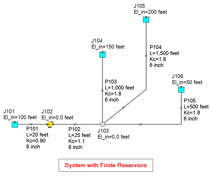
Figure 1 - System with Reservoir Junctions using the Finite Open Tank model option when using the AFT Fathom XTS module.
Table 1 contains the finite tank input for the reservoir junctions. All tanks are 100 ft tall, open to atmospheric pressure, and the discharge tanks are initially empty.
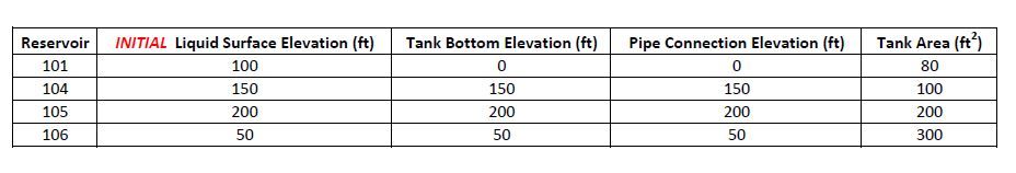
Table 1 - Finite tank junction input information. All tanks are 100 ft tall, open to atmospheric pressure, and initially empty (except for J101 which is initially full).
I ran a 10-minute transient simulation with 15 second time steps. The pump operates continuously at 100% speed. The supply tank drains while the empty discharge tanks fill. Figure 2 shows the change in liquid height over time for each tank. As Liquid Surface Elevations change, so will the static head. Remember that the static head is not simply the difference in liquid surface elevations, as discussed in the previous Part 2A blog.
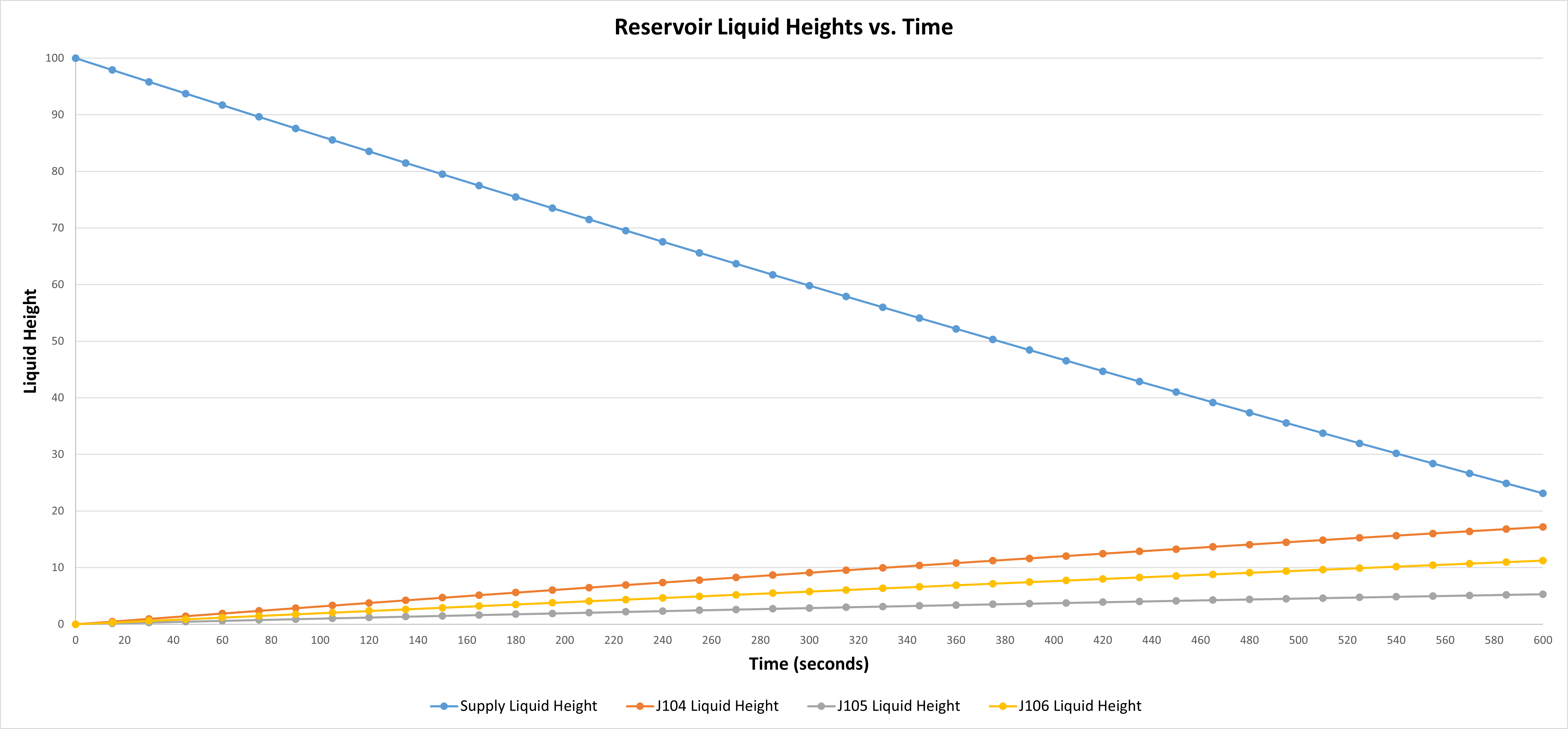
Figure 2 – Reservoir junction liquid height vs. time for supply and discharge tanks of multi-branched system.
"Know Your Pump & System Curves – Part 1", showed how to calculate static head. In "Know Your Pump & System Curves – Part 2A", we saw calculating static head for a multi-branched system like this is more complicated. The numerical value of static head and the shape of the system curve depends on if reverse flow into the piping system from the discharge tanks is allowed or not when generating the system curve. The system in Figure 1 does not have any check valves present. Therefore, the potential for reverse flow is allowed at lower pump-driven flow rates when generating the system curve.
How would you generate a system curve and calculate static head for a system like this that is constantly changing? Follow the same process outlined in the previous blogs. Using AFT Fathom to generate the system curve for a transient simulation will only generate a curve for the initial state of the system at time zero. To create a "transient system curve", you could use AFT Fathom to generate a series of system curves at different time data points. Each system curve represents a specific snapshot in time.
From Figure 2, we know how the Liquid Surface Elevation for each tank changes. Table 2 shows the liquid surface elevation for each tank every 2.5 minutes. This data serves as the input boundary conditions at each time step for the reservoir junctions so that AFT Fathom can generate a system curve in the normal fashion at each time step.
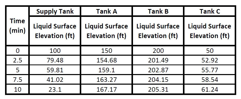
Table 2 - Liquid Surface Elevation data for each tank every 2.5 minutes.
In Figure 3, the "System with Finite Reservoirs" shown from Figure 1 was duplicated several times to create six nearly identical multi-branched systems on the same Workspace. The first five systems are modeled using the Infinite Reservoir model and for the system that represents each time step, the appropriate Liquid Surface Elevation from Table 2 for each reservoir junction was specified as input.
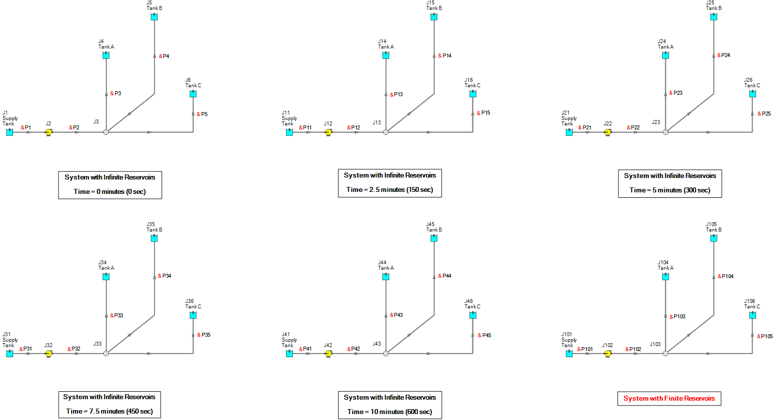
Figure 3 - Five multi-branch systems using Infinite Reservoir model with Liquid Surface Elevations specified as input for each snapshot in time. Liquid Surface Elevations were calculated from the System with Finite Reservoirs during the transient simulation.
The five systems using Infinite Reservoir models allow the pump and system curve to be calculated for each snapshot in time every 2.5 minutes for the 10-minute transient simulation. Figure 4 illustrates each system curve at every 2.5 minutes plotted together against the pump curve (which remains at the same operating speed for the whole transient simulation). Included on this plot is the pump efficiency curve, the BEP clearly identified, and the Preferred Operating Region (POR) labeled as well.
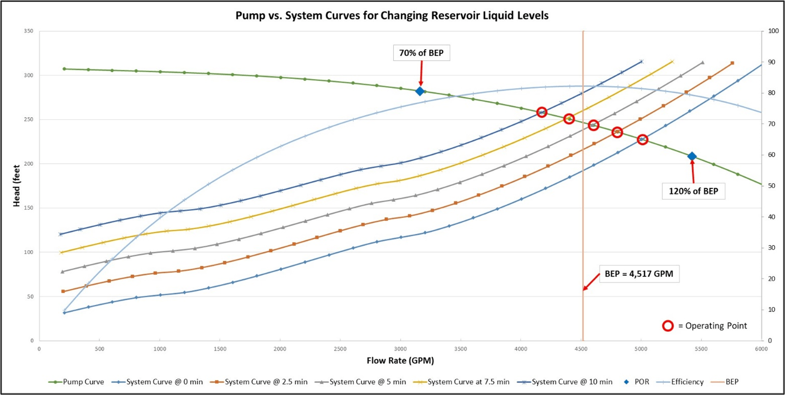
Figure 4 - Multiple system curves plotted against pump curve to illustrate a "transient system curve" that changes over time.
The system curve at time zero is the same system curve that was generated in the previous (Part 2A) blog for a multi-branched system without check valves. The system curve generation method for the curves at each time step allows the possibility of reverse flow at lower pump flow rates as well. Notice how the system curve shifts such that the pump continues to operate further back on its curve at lower and lower flow rates. As the static head increases during this process, the pump must provide more Total Dynamic Head to overcome larger differences in elevation between supply and discharge.
The important thing to take away from the plot in Figure 4 is essentially where the pump is operating during the transient simulation in relation to its BEP. For this system, the pump still operates within very close proximity to its BEP, and clearly well within the bounds of the POR. Pumps that are not sized properly for a system may exceed the POR boundaries and this can cause significant reliability issues when operating far away from BEP.
Thought it could not get any more complicated? How about a multi-branched system with a fourth branched flow path with a second pump like in Figure 5? In this system, the design flow rate for pump J2 is 10,000 GPM while the design flow rate for pump J7 is 3,000 GPM.
What is the system curve for this piping system? As discussed earlier and in the previous blogs, this is another example where a single unique system curve representing the overall system resistance does not exist. Let us consider the reference point of each pump in Figure 5 to generate a system curve. Note that the check valves in Figure 5 have been failed open for modeling purposes. Therefore, in the potential for reverse flow through the branch flow paths, these check valves will not close. Figure 6 represents the pump and system curve for pump J2 and J7 when the possibility for reverse flow is allowed during the system curve generation process.
Obviously, the system curves for each pump are quite different from each other.

Figure 5 – Multi-branched system with fourth branched flow path including a second pump. Pump J2 design flow rate is 10,000 GPM while pump J7 design flow rate is 3,000 GPM.

Figure 6 – Pump and system curves for pumps J2 and J7 of multi-branched system with four flow paths and two pumps in different locations. Each individual pump efficiency curve and POR points included.
We now understand how the curves from Figure 6 are easily generated in AFT Fathom. However, when AFT Fathom generates the system curve for either pump, what is the other pump doing during the system curve generation process? The simple answer is that the other pump just operates on its pump curve that was entered into the pump model. This can be demonstrated using the AFT Fathom XTS module, like the approach in the previous example to create the "transient" system curve of Figure 4. But this time, the reservoir junctions in Figure 5 use the Infinite Reservoir model and thus, the liquid levels will not change.
Note that the transient analysis discussed next is not intended to represent the transient dynamics of a real system. It is simply intended to help illustrate what is happening with both pumps as AFT Fathom generates the system curve for each individual pump. Also note that in this "transient" analysis, the check valves can function as actual check valves where they will be closed if there is any reverse flow in the branch flow paths at a given time step. The system curves that will be generated "manually" with the transient analysis here will not completely match the system curves shown for each pump in Figure 6 due to the function of the check valves.
This will help you understand what AFT Fathom is doing when you generate a system curve for a specific pump in a more complicated system with multiple pumps in different locations. I do not mean multiple pumps in parallel or series in this case. That will be discussed in the next blog.
The first transient analysis models pump J2 as a fixed flow pump. The flow increases linearly from 0 – 12,000 GPM over 240 seconds. The pump head required to deliver a flow at a given time step to overcome system resistance and elevation change will be calculated. This will determine a "system curve" manually for pump J2. Pump J7 will operate on its specified pump curve model.
Figure 7 is the transient flow vs. time data plotted for each of the pumps. Figure 8 is the pump flow vs. head plotted for the pumps at each time step. Here, you can see that when the pump head for J2 is calculated for a range of flow rates when generating the J2 system curve, pump J7 is simply operating on its own curve at whatever the flow rate through J7 would be at a given time step.
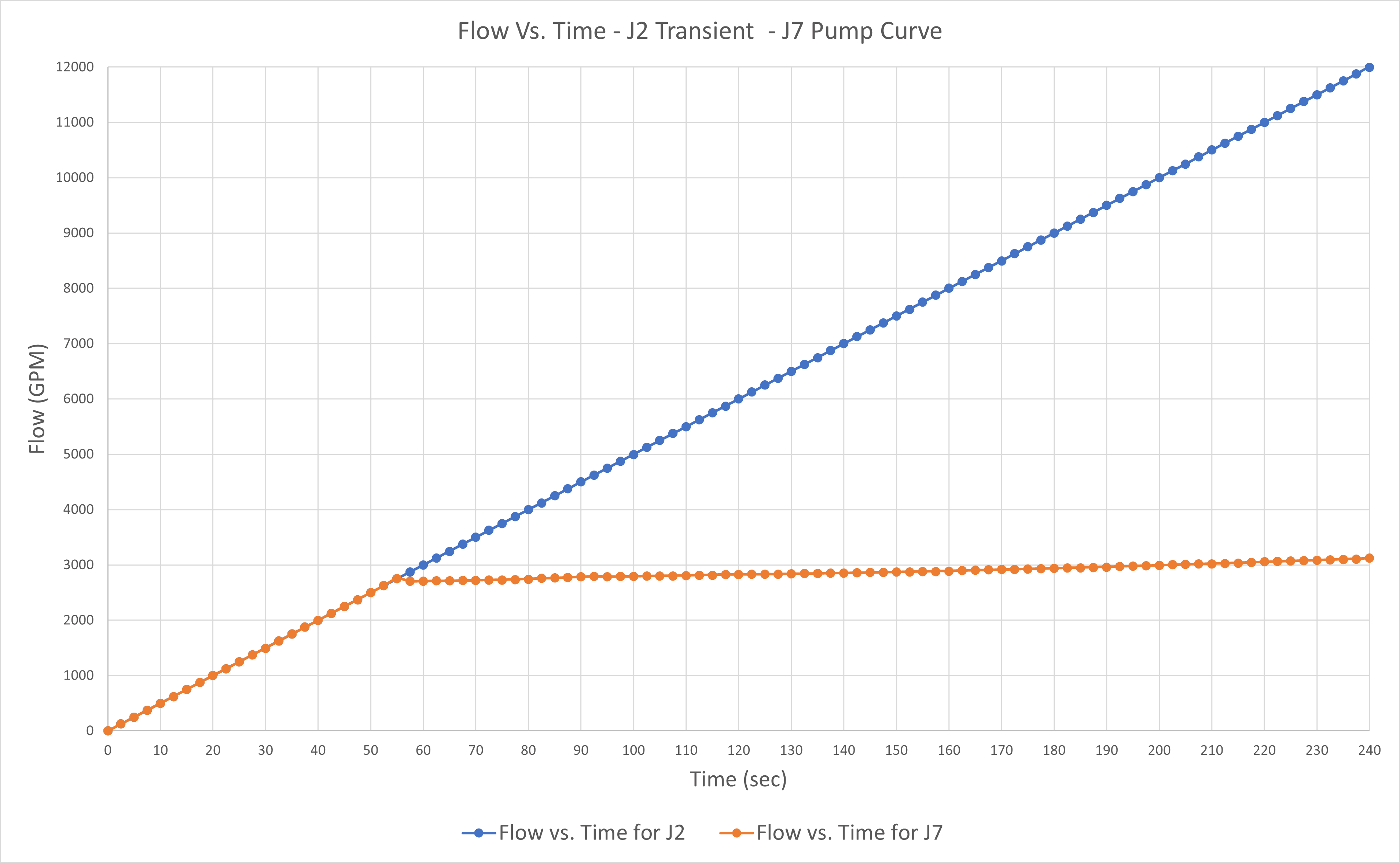
Figure 7 - Flow vs. Time data for pumps J2 and J7. Flow changes linearly with time through J2 while J7 operates on its pump curve.
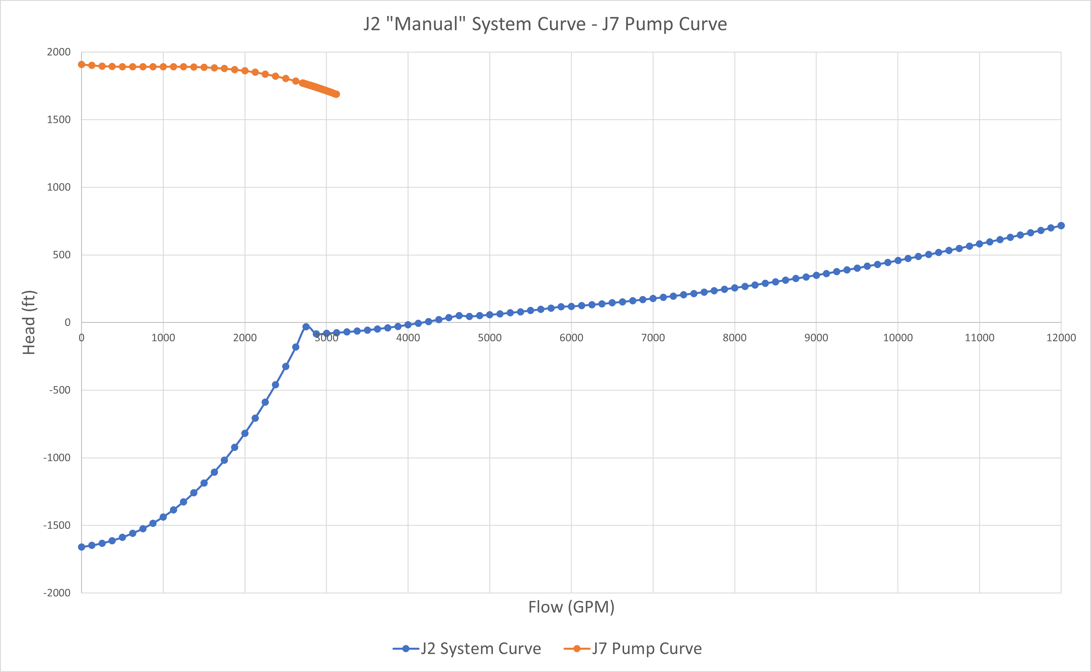
Figure 8 – Pump head vs. flow for pumps J2 & J7. J2 represents a system curve at J2 for a range of flow rates with J7 shown to operate on its curve during a system curve generation process of J2.
The second transient analysis models pump J7 as a fixed flow pump. The flow increases linearly from 0 – 4,000 GPM over 240 seconds. The pump head required to deliver a flow at a given time step to overcome system resistance and elevation change will be calculated. This will determine a "system curve" manually for pump J7. Pump J2 will operate on its specified pump curve model.
Figure 9 is the transient flow vs. time data plotted for each of the pumps. Figure 10 is the pump flow vs. head plotted for the pumps at each time step. Here, you can see that when the pump head for J7 is calculated for a range of flow rates when generating the J7 system curve, pump J2 is simply operating on its own curve at whatever the flow rate through J2 would be at a given time step.
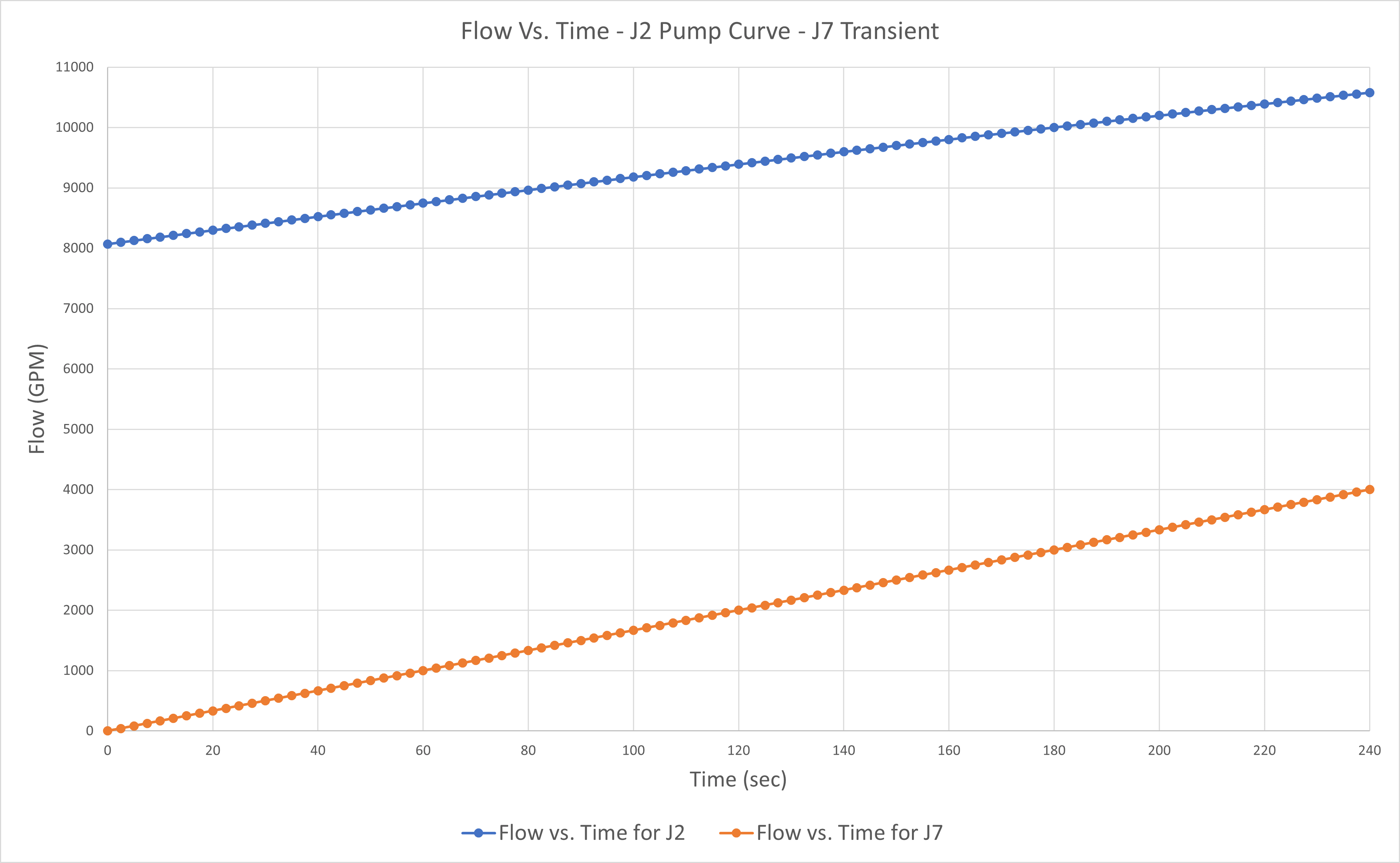
Figure 9 - Flow vs. Time data for pumps J2 and J7. Flow changes linearly with time through J7 while J2 operates on its pump curve.
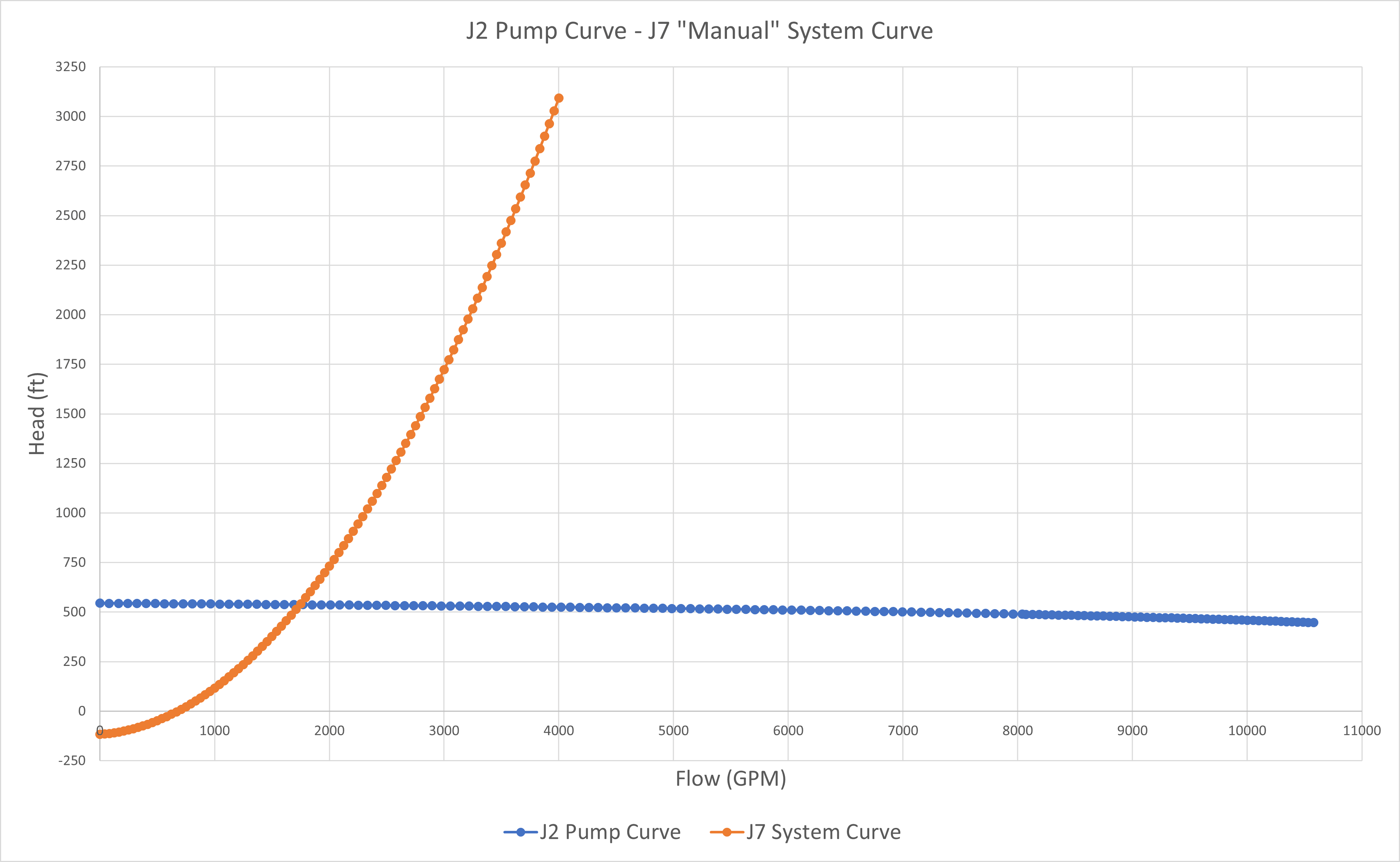
Figure 10 - Pump head vs. flow for pumps J2 & J7. J7 represents a system curve at J7 for a range of flow rates with J2 shown to operate on its curve during a system curve generation process of J7.
Here is another good example of the case of generating pump and system curves for a complicated system with multiple pumps in different locations of the system. Refer to the model in the case study AFT Fathom Used to Enhance 40-Year Old Hand Calculations at Nuclear Power Plant. There are four pumps that are in different parts of the system. So, whenever a pump vs. system curve is created for a specific pump in this model, all the other pumps are simply operating on their individual curves while the system curve for a specific pump is generated.
In conclusion, we took a deeper look at pump vs. system curves for complicated multi-branched systems. We evaluated a case to demonstrate how the system curve changes over time during a tank filling process while the supply tank drains. The key thing to focus on there is how the operating point changes over time in relation to the BEP. As the operation gets further outside the Preferred Operating Region, more reliability issues may become present.
The other case we looked at was like the previous multi-branched system but contained a fourth branched flow path which included a second pump in the system. Pump and system curves were generated for this system as well and it is important to pay attention to where each pump operates with respect to its own BEP. But the focus in the second case was to illustrate deeper what is happening to other pumps in a system when generating a system curve for a specific pump. As shown, they are operating on their own pump curves, and this will have an impact on the system resistance that each individual pump needs to compete against.
Stay tuned for the final blog article in the series that will discuss pump and system curve interaction with multiple pumps in series or parallel configurations.
Comments