


AFT Blog
Welcome to the Applied Flow Technology Blog where you will find the latest news and training on how to use AFT Fathom, AFT Arrow, AFT Impulse, AFT xStream and other AFT software products.
19 minutes reading time
(3855 words)
Featured
What Is Transient Analysis?
You're tasked to perform a transient analysis of a piping system and it would be really helpful if there was a good software tool out there to help you. Well, you've come to the right place because AFT has great solutions! But our first question is, "What kind of transient analysis are you trying to do?" You might start scratching your head thinking, "There's more than one???"
Yes there is, and which type of transient analysis you need to perform depends on the context of what you are trying to study. Do you want to know how long it tanks to fill up a tank? How changing user demands throughout the day affects pump performance and system interactions? Or are you trying to figure out what kind of pressure surge you might see from a sudden valve closure? Or are you looking to see if cavitation is present during a pump shut-down?
These and many other questions like this require different solutions for the transient analysis you are trying to do. Should you use AFT Fathom's eXtended Time Simulation (XTS) add-on module or should you be using AFT Impulse? Or do you need both?
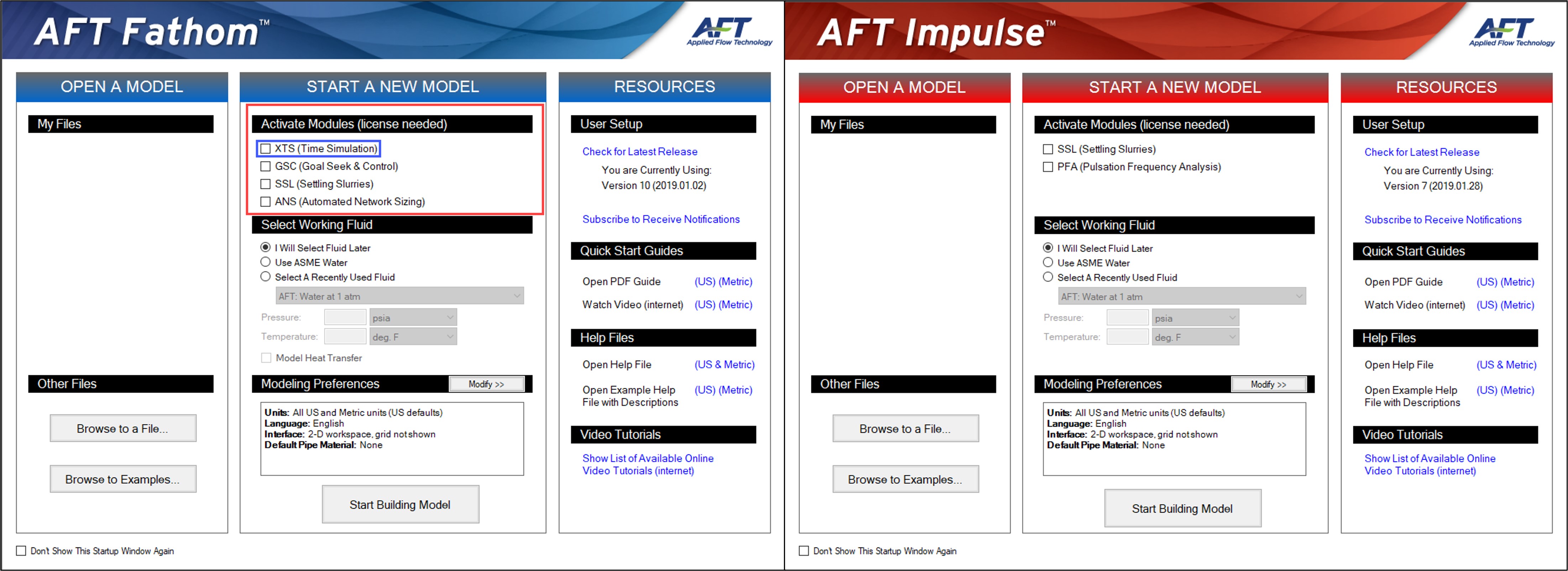
AFT Fathom XTS Module vs. AFT Impulse. Which do you need?
An important point to note is that a major advantage is the interface and modeling process for all AFT software products is virtually identical. Also, you can easily open any AFT model built in a particular AFT software product in another AFT software product! So, if you have an AFT Fathom model where you finished your steady-state or transient analysis with the AFT Fathom XTS module, you can then open your model in AFT Impulse so you can do your waterhammer/surge analysis.
This blog article is going to present an example of an application where you could (and probably should) use BOTH the AFT Fathom XTS module AND AFT Impulse for a transient analysis. I will also provide examples of different types of questions that you might ask which would lead you to when you would use AFT Fathom's XTS module compared to when you would use AFT Impulse.
A helpful way to understand when to use AFT Fathom XTS vs. AFT Impulse is to think "Long Term Simulation" vs. "Short Term Simulation". The AFT Fathom XTS module would be used for doing a "Long Term" transient simulation over long periods of time from several minutes, to hours, perhaps even days. You would be trying to focus on how the system interacts with itself over long periods of time. A key assumption using the AFT Fathom XTS module is that every time step is a steady-state solution. This assumption may be valid over long periods of time where at a particular snapshot in time would reflect a steady-state operation if no other changes were occurring. Time steps are often ranging from 30-60 seconds up to several minutes long depending on how long the transient duration is. Between longer-duration time steps, it is possible that any pressure and velocity waves that would be present during a sudden surge event may have dampened out if the system is changing slowly in this way.
AFT Impulse models a transient simulation for what happens after a sudden surge or waterhammer event. Simulation time periods are very short. Often several seconds to maybe a minute or two. A few minutes at most would be a very long transient simulation period in AFT Impulse. The time steps in AFT Impulse are very short, on the order of milliseconds. AFT Impulse will track how fast a surge/waterhammer wave (for pressure and velocity) propagates through a system according to its wavespeed before the surge waves eventually dampen out as the system has approached a new steady-state operation. The key description for "waterhammer" is essentially the process a piping system undergoes as it transitions from one steady-state operation to another steady-state operation. With wavespeeds on the order of typically several thousand feet per second, surge/waterhammer transients occur very fast and AFT Impulse captures the fast transient behavior where the AFT Fathom XTS module does not.
In summary, think "Slow Transients" with the AFT Fathom XTS module and "Fast Transients" for AFT Impulse.
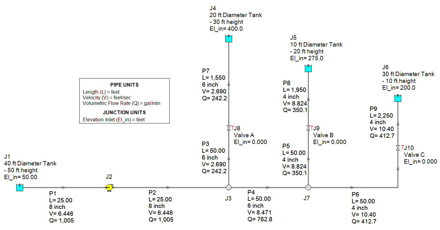
Figure 1 - AFT Fathom model using the
eXtended Time Simulation (XTS) module to determine how long it takes to fill up the tanks and when valves will close to prevent overfilling in multi-tank filling application.
I'm going to start with a simple multiple tank filling application using the AFT Fathom XTS module. In the system shown in Figure 1, there are three discharge tanks that are initially empty, each at different elevations and with different diameters. A major advantage using the AFT Fathom XTS module is that you can model finite open and closed tanks.
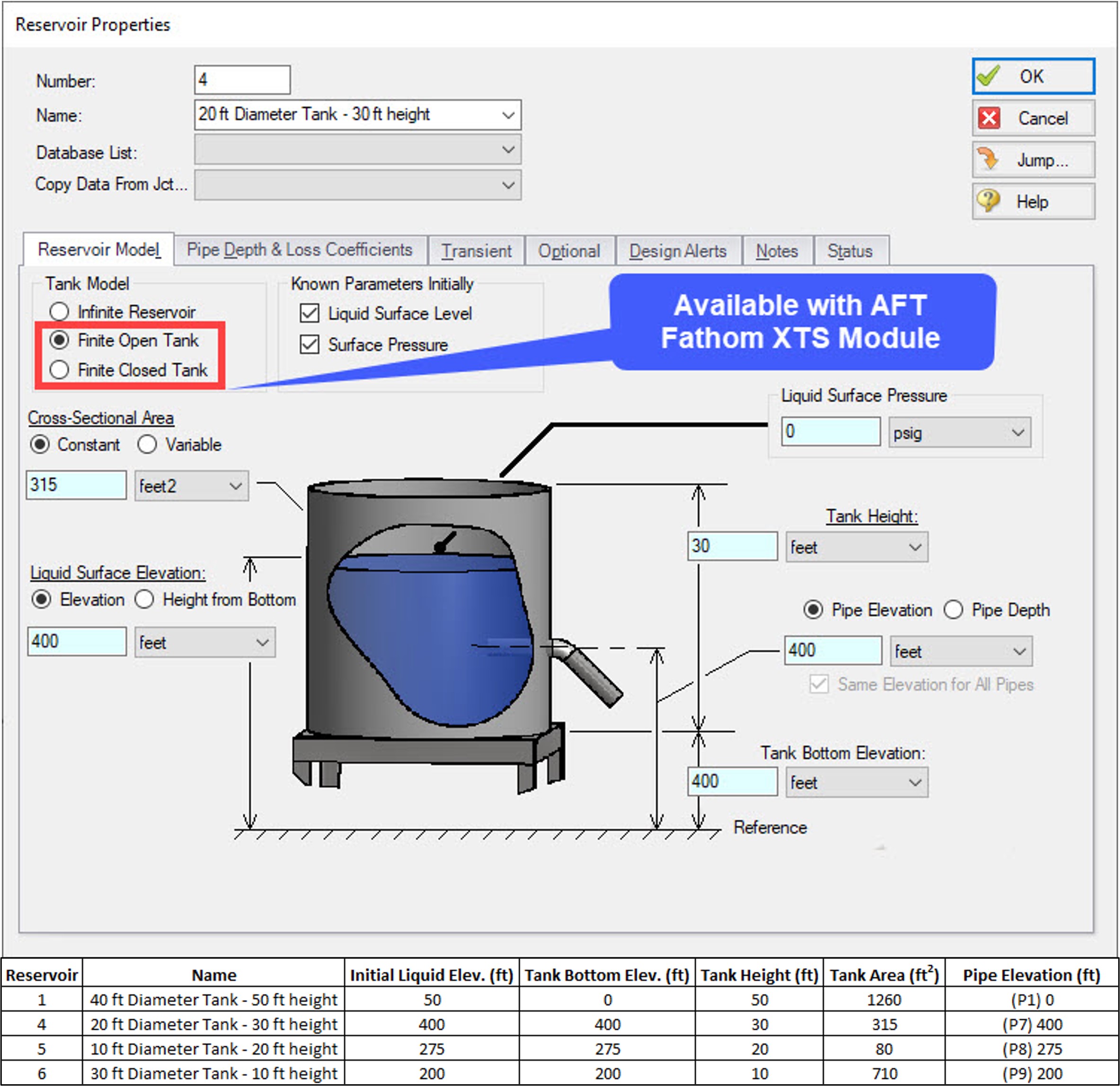
Figure 2 - Reservoir Property window for modeling Finite Tanks with AFT Fathom XTS module. Finite tank input for Reservoir junctions in Figure 1 included.
In standard AFT Fathom without the XTS module, Reservoir junctions represent infinite sources or sinks of fluid that will maintain a fixed pressure at a pipe connection. The liquid levels will not change unless it is changed manually by the user. So, using the AFT Fathom XTS module brings helpful benefits for modeling tanks and Figure 2 provides an example of what the Reservoir junction Property window looks like when choosing a finite tank option.
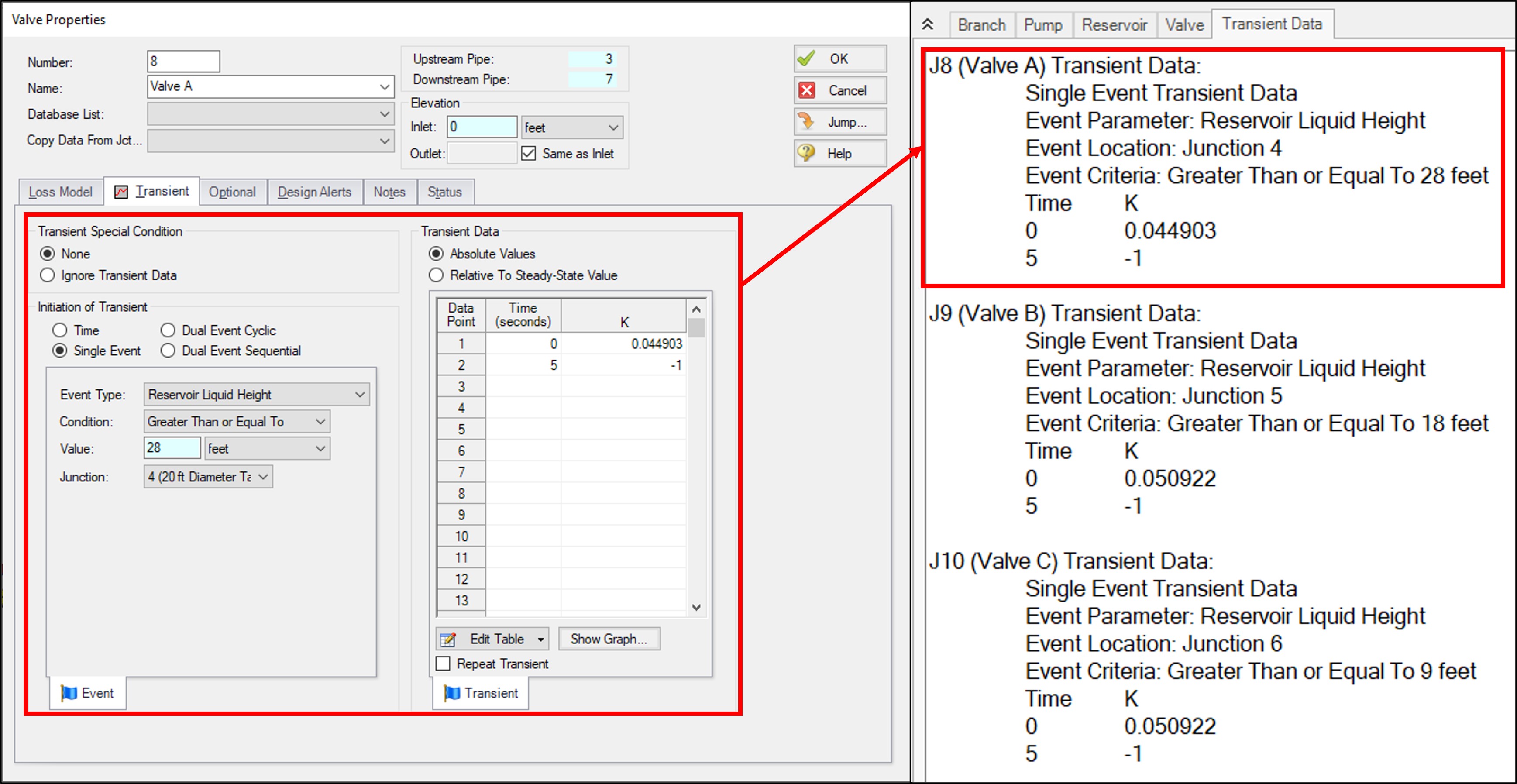
Figure 3 - Single Event Transient to close the valve based upon Reservoir Liquid Height Criteria. Transient Data profile defined to close the valve within five seconds.
It is important that the tanks do not overfill. A transient event will close the valves once the liquid level in each respective tank reaches a certain level. A "Single Event" type of transient is going to be used for this where the valve will close at a rate defined by the Transient Data profile. The Single Event transient requires that criteria must be met for the valve closure to activate. The event condition will be when the Reservoir Liquid Height gets to be within one or two feet of the top of the tank, as shown in Figure 3.
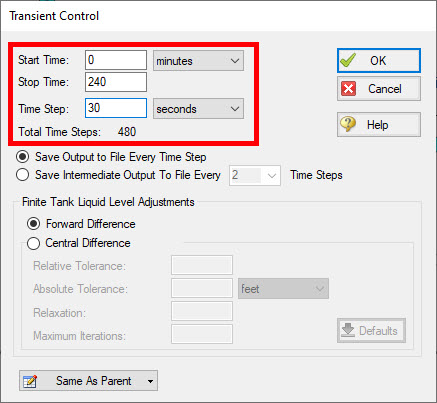
Figure 4 - Transient Control for AFT Fathom XTS tank-filling transient simulation. Four hour long (240 minute) duration with 30 second time steps.
The last thing to specify for the AFT Fathom XTS simulation is the Transient Control shown in Figure 4. This is where you specify how long the transient simulation will be for. This example is going to run a four hour long (240 minute) duration with a time step of 30 seconds which will yield 480 Total Time Steps.
Notice how the valve closure rate takes place in less time than the defined time step (5 second closure rate vs. 30 second time step). Any event that happens in a time frame that is less than the defined time step is essentially "instantaneous". In reality, sudden events will cause waterhammer/surge waves to propagate through the system at the speed of sound. This is not captured with the AFT Fathom XTS module and needs to be evaluated with AFT Impulse.
You have the flexibility to change the time step directly in the AFT Fathom XTS module. This is not the case with AFT Impulse and is a key difference between the two types of transient analysis. In AFT Impulse, the time step is determined through sectioning the pipes for the Method of Characteristics which solves the network of the transient mass and momentum balance equations.
This is very important to look deeper into because if a valve closes in five seconds and causes very large pressure waves that are propagating through the system and interacting with other transients. These transients are happening very fast, and they will be completely missed for two reasons. First, the 30 second time steps do not provide the resolution. Second which is a bigger issue is that the wavespeed is not accounted for in long term transient analysis with the AFT Fathom XTS module where each time step is assumed to be a steady state. Therefore, AFT Impulse is needed and will be demonstrated later in this article.
Here are some basic examples of questions that might be asked for a "long-term" type of transient analysis with the AFT Fathom XTS module.
- How long does it take to fill the tanks and when do the valves close?
- How do the tank liquid levels change over time?
- How does the pump operation change over time for flow, pump head, BEP proximity, suction & discharge pressure?
- What are the pressures at the valve over time? Specifically at the time of valve closure?
- How does the pressure change throughout the system over time?
Figure 5 shows the Event Messages By Time which easily answers the question of what time the valves close, which is confirmed by the Cv vs. time profiles as well. As you can see, the closure times are very different based upon the individual flow paths and specifications of each tank.
The changing liquid levels is given by the graph in Figure 6. Notice how the tank fill rates change in slope as valves are closed.

Figure 5 - Event Messages By Time identifies valve closure times and is confirmed by valve Cv vs. Time profiles.
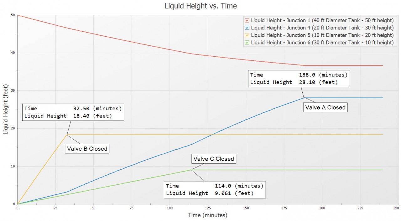
Figure 6 - Changing liquid heights vs. time for each tank. Tank levels reach a constant value once the valve leading to it is closed.
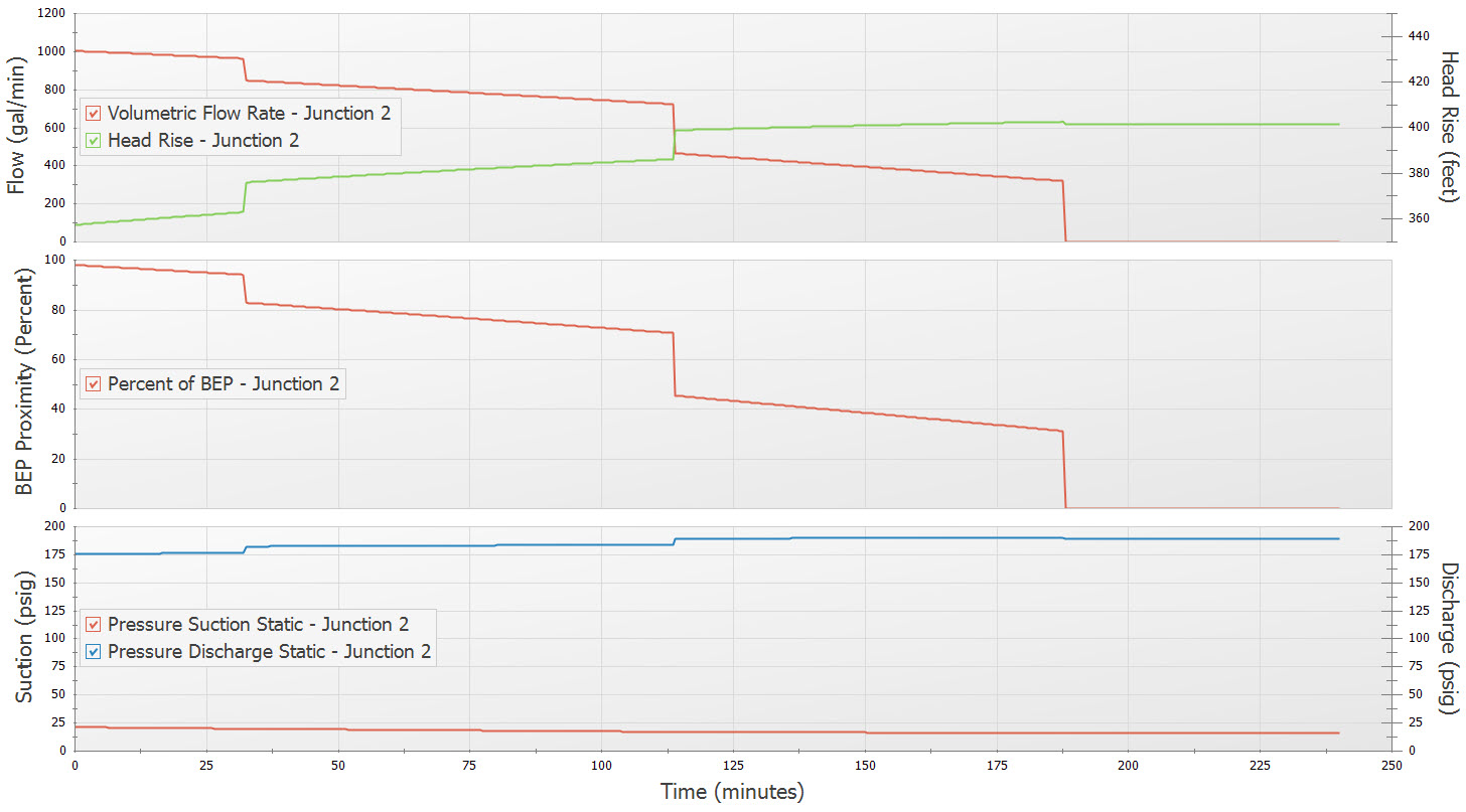
Figure 7 - Pump operation vs. time for flow, pump head, BEP proximity, suction, and discharge pressure. Notice the very low BEP proximity operation for about 75 minutes after two of the valves have closed, which can lead to pump reliability issues.
The transient pump operation for flow, pump head, Best Efficiency Point (BEP) proximity, suction, and discharge pressure is shown in Figure 7. Notice how the decreasing flow through the pump causes it to ride further back on its curve at higher pump heads. Once two of the valves have closed, you can see how the BEP proximity significantly drops to between 45% to 30% for just over 70 minutes. Not an operation that you want to maintain for a long period of time. If the pump was experiencing problems, this could help explain why.
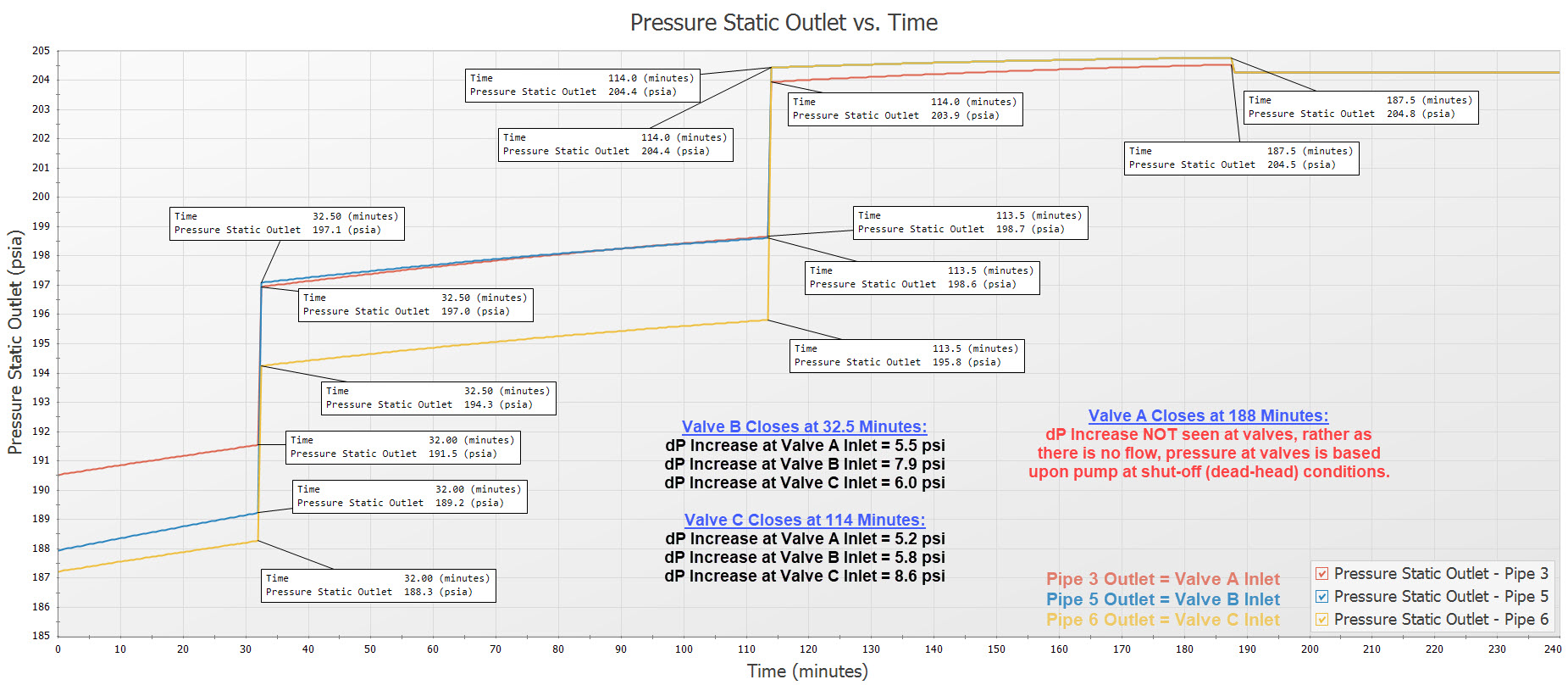
Figure 8 - Valve Inlet pressure for each valve during AFT Fathom XTS transient simulation. Note the pressure increase at each valve upon valve closure. When the final valve closes, valve inlet pressures DECREASE to the shut-off pressure of the pump.
Now let's take a look at the pressures at the valves during the simulation shown in Figure 8. This is a plot of the outlet pressure of the pipes, which corresponds to the inlet of the valves. The important thing to focus on here is the increase in pressure at each valve, any time one of the other valves close. For example, Valve B (plotted in blue) closes first at 32.5 minutes into the simulation. Keep in mind that the valves take five seconds to close and the time step is 30 seconds. When Valve B starts to close, the pressure is 189.2 psia and once it is fully closed, the pressure is 197.1 psia. A pressure increase of 7.9 psi.
Another thing to notice in Figure 8 is at 187.5 minutes when Valve A closes. The pressure at the valve inlets DECREASES! The pressure decreases to what the dead-head/shut-off pressure is when the pump operates at zero flow. It is interesting that we do not see an increase in pressure at the valves in this case.
Figure 9 is an animated video of the pressure profiles from the supply tank to each discharge tank through the respective flow paths. When you play this animation, you can see how the pressure changes throughout the entire system over time. Watch how the pressure changes abruptly at the time for each valve closure event.
With the AFT Fathom XTS module, we were able to determine how long it takes to fill up the discharge tanks as well as how fast the supply tank will drain. The simulation also showed what time the valves will close and how the pump performance changes over time.
But the big question is…are the pressures we are seeing realistic? Waterhammer events caused by things such as sudden valve closures can cause very large pressure surges in piping systems that can destroy piping and equipment. If we only consider the pressures we see in Figures 8 and 9, we may not be very concerned. However, quick research of waterhammer literature shows how catastrophic these events can be.
This is where I will now shift the focus to AFT Impulse and how it can be used to model waterhammer/surge transients in piping systems. As described earlier, AFT Impulse models transients caused by SUDDEN or "instantaneous" events. The "short term" transient simulation we will model will be completed in three different scenarios. We are going to evaluate what happens in the system at each closure event and will run a 90 second simulation for each scenario. Note that this is equivalent to three time-steps of the AFT Fathom XTS simulation.
- Scenario 1: Valve B closes in five seconds while the other valves are fully open
- Scenario 2: Valve C closes in five seconds while Valve B is already closed & Valve A is still open
- Scenario 3: Valve A closes in five seconds while Valve B & C are already closed
In AFT Impulse for scenarios 2 and 3, we will model the valves already closed as Dead-End junctions because they will simply act as reflecting points in those scenarios. This will help simplify the model for those scenarios. Figure 10 shows the AFT Impulse model Workspace for each transient scenario.
Figure 10A - AFT Impulse model for Scenario 1 at 32 minutes from AFT Fathom XTS simulation. Valve B closes in five seconds while Valves A & C remain Open.
Figure 10B – AFT Impulse model for Scenario 2 at 113.5 minutes from AFT Fathom XTS simulation. Valve C closes in five seconds, Valve B already fully closed & modeled as Dead-End Junction, & Valve A remains fully open.
Figure 10C – AFT Impulse model for Scenario 3 at 187.5 minutes from AFT Fathom XTS simulation. Valve A closes in five seconds while Valves B & C already closed & modeled as Dead-End Junctions.
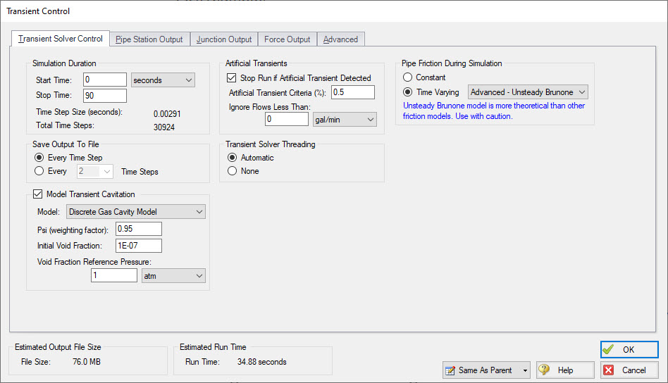
Figure 11 - Transient Control window for AFT Impulse. Time-step is 3 milliseconds with a 90 second simulation period
Waterhammer/surge events can also be known as "fast transients". The amount of time it takes a transient pressure wave to propagate and communicate its presence to the rest of the systems occurs in a very short time frame. This is because the wavespeed of the fluid is on the order of a few thousand feet per second. For example, the wavespeed for an 8-inch nominal size STD (schedule 40) steel pipe that is thick-walled and anchored upstream is about 4,200 feet/second. Therefore, surge waves travel FAST!!
To capture this fast transient behavior, we need a very small time-step which is typically on the order of a few milliseconds. As mentioned earlier, the time-step in AFT Impulse is not specified directly, rather it is determined through pipe sectioning. After the pipes have been sectioned, the Transient Control is specified as shown in Figure 11. As you can see, the time-step for this waterhammer analysis is about 3 milliseconds. In a 90 second simulation, there are almost 31,000 time-steps. The Transient Control window for AFT Impulse is much more complex than the Transient Control window for the AFT Fathom XTS module because there is a lot more complexity going on behind the scenes in the calculations for AFT Impulse than with the AFT Fathom XTS module.
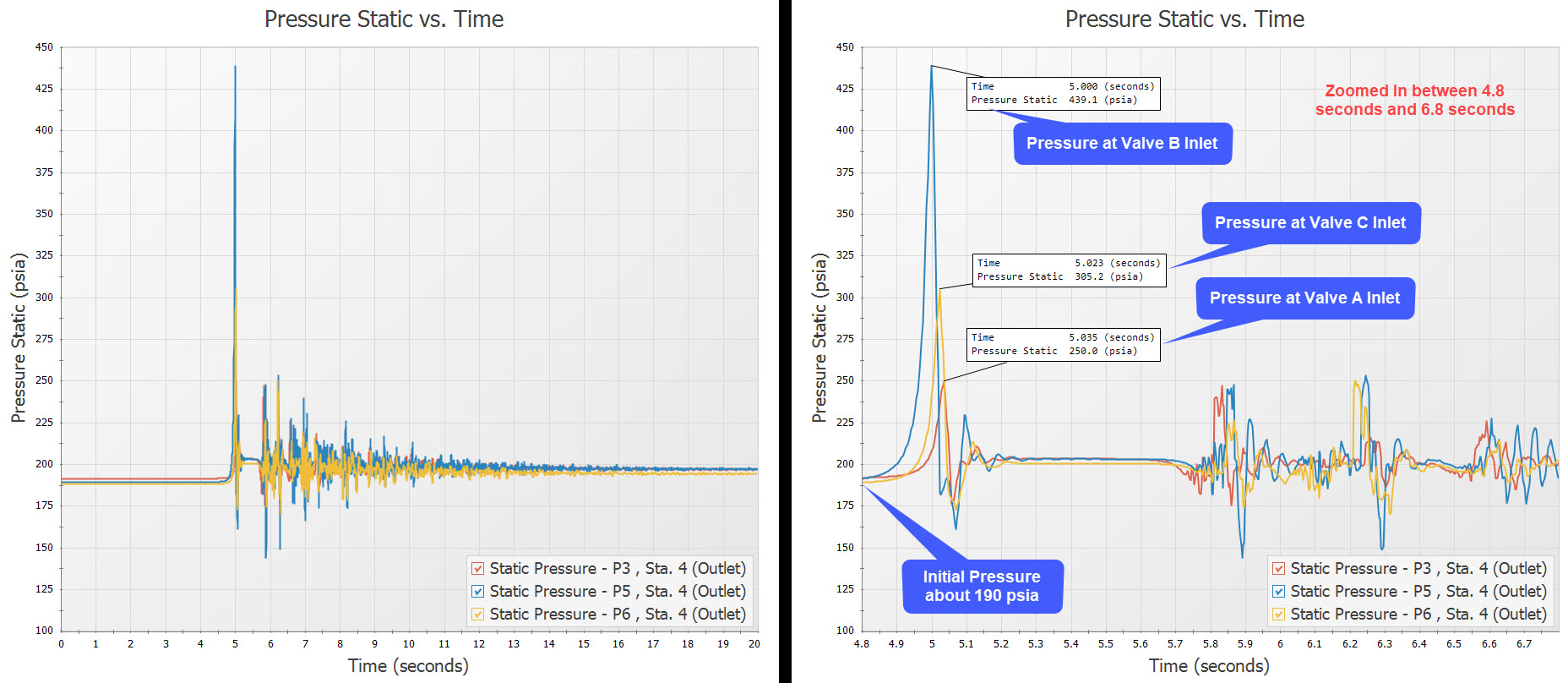
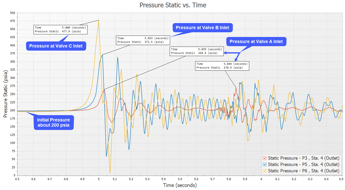
Figure 12 - AFT Impulse Scenario 1 transient pressure at valve inlets. Valve B closes, causing large spikes in pressure. Graph on the right is zoomed in to between 4.8 seconds to 6.8 seconds.
AFT Impulse is going to evaluate exactly what happens at the moment of valve closure and shortly after. Here is an example of some questions you might ask when considering a waterhammer analysis with AFT Impulse.
- How large are the pressure spikes upon valve closure?
- Is cavitation present in the system & if so, what are the pressure magnitudes on vapor collapse?
- What happens to the system pressure during a pump trip event?
- How do check valves, relief valves, or control valves respond during a sudden event? Can they maintain control in realistic time frames or do they fail or chatter?
- What type of surge suppression equipment is needed to protect in a sudden surge event?
For the sake of simplicity, this blog will focus on the transient pressures at the valves as well as how the pressure surges through the piping system. Also, after running the first two scenarios, I found that the transients had all dampened out within the first 30 seconds of the simulation. So, I will only focus on the results within that short time frame. The last scenario is a different matter and will get to that shortly.
In Scenario 1, a large pressure surge is going to occur at the inlet of Valve B once it is closed and will then propagate through the rest of the system. Figure 12 shows the transient pressure at the inlet to each valve in the first 20 seconds of the simulation. The graph on the right in Figure 12 is zoomed into the timeframe between 4.8 seconds to 6.8 seconds to highlight better the pressure spikes upon valve closure. First off, the pressure surge at the inlet of Valve B rises to about 440 psia when it closes. The 250 psi increase in pressure is astronomical in comparison to the 7.9 psi increase with the AFT Fathom XTS module!
The animation in Figure 13 shows how the sudden valve closure of Valve B causes a large surge pressure that is transmitted everywhere else in the system. Very quickly, the other flow paths through Valves A and C experience the large surge pressure caused by Valve B when it is closed. Notice how the pressure wave passes through the system. The end of the flow paths through Valve A & C right near the tanks do experience cavitation and when the vapor cavities collapse, this causes additional pressure spikes that can be quite severe. You can also see how pressure waves begin to interfere with each other both in constructive and destructive interference patterns. This can also cause large pressure spikes at times.
A much deeper analysis of this phenomenon is required, especially due to the presence of cavitation. The important take-away here is to see how the pressure surges are much higher when properly predicted using the Method of Characteristics for a waterhammer analysis and how these pressure waves are quickly transmitted through the rest of the system.

Figure 14 - Transient pressure at Valve Inlets for Scenario 2 of the AFT Impulse transient simulation where Valve C closes linearly in five seconds. Note the initial pressure is about 200 psia, about 10 psi higher than Scenario 1.
Figure 14 provides the transient pressure at the valve inlets for Scenario 2 where Valve C closes linearly in five seconds while Valve B is already closed and modeled as a dead-end junction. Note how the initial pressure is about 10 psi higher in Scenario 2 than Scenario 1. This is because not only are different valves closing in different scenarios, but the initial conditions for the tanks are different in each scenario. This is where the AFT Fathom XTS module is very helpful because at the time-step in the XTS simulation where the tanks start to close, we can easily get the resulting liquid height and use it as an input for the AFT Impulse analysis.
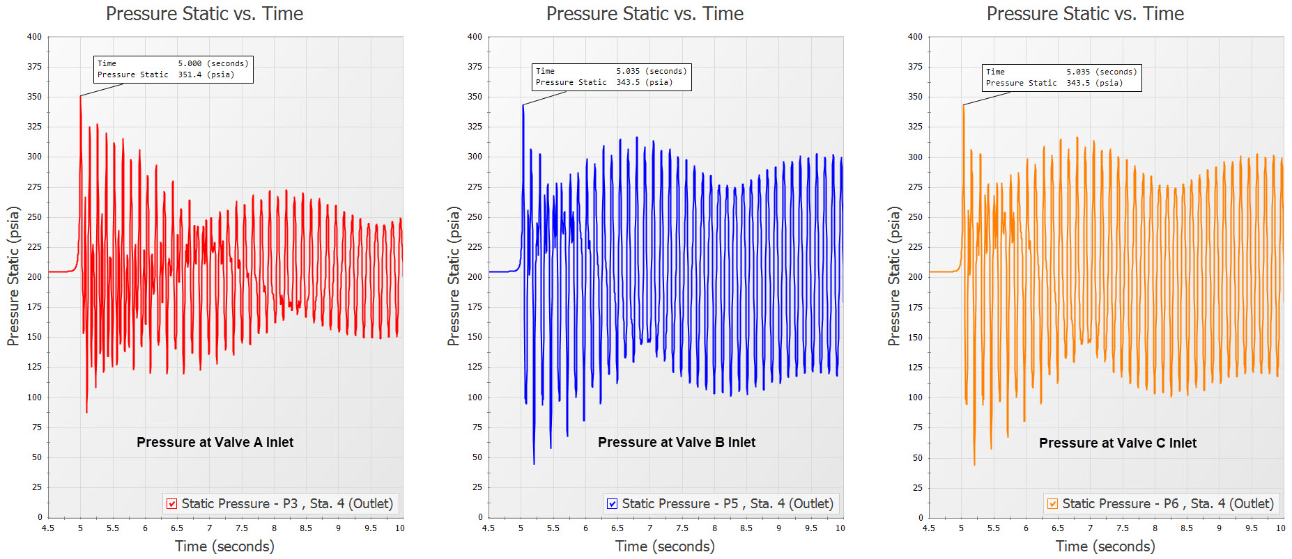
Figure 15 - Pressure transients at valve inlets for the Scenario 3 linear closure of Valve A with Valves B & C already closed. Much shorter flow paths to closed flow paths and pump operating at dead-head conditions leading to significant pressure oscillations.
An animation for Scenario 2 would be slightly different because as Valve C closes and Valve B is already closed, there is now a NEW reflecting point for the system at closed Valve B. Therefore, there is not as much distance for the transient waves to travel in the system. This will change the reflective behavior in the system which can cause larger and smaller pressure spikes and different wave interference patterns.
Scenario 3 closes Valve A linearly in five seconds and Valves B & C are fully closed and are modeled as dead-end junctions. In this system, there is much less distance that waves have to travel since the closed Valves B & C have closed off the flow paths. The pipe lengths to each of the valves is only 50 feet while there was much more distance of piping downstream of the valves. Therefore, once Valve A is fully closed, there is going to be much more significant oscillation in this system because the transient waves are "trapped" in a much smaller amount of space. Figure 15 is a plot of the pressure at the valve inlets from 4.5 to 10 seconds of the simulation for the Valve A closure.
This level of significant pressure oscillation can potentially cause severe damage to a system, especially if it takes a while for the transient waves to dampen out. The pump continuing to operate at dead-head conditions also leads to this level of oscillation. Therefore, the next scenario to evaluate would be to then trip the pump to avoid dead-heading against closed valves. This scenario will not be evaluated for this blog article. But as you can see, there is a LOT to evaluate when it comes to waterhammer analysis.
In conclusion, transient analysis is very important to evaluate for piping systems and there are two types of transient simulations. A long-term transient using the AFT Fathom XTS module which looks at the system dynamics over long periods of time while a short-term transient simulation using AFT Impulse looks at what happens in the very short time-frames during a waterhammer/surge event which accounts for the rapid propagation of transient pressure waves through the system at thousands of feet per second. Both types of transient analysis have great areas of application and need, and this blog article provided one specific example.
Comments