Flow Coefficients and Loss Factors: Valve Transients

It is well-known that valve closures and openings can cause waterhammer events. Because this is perhaps the most common cause of surge events, it is important to understand how to input valve transients and characteristics.

Regarding both steady state characteristics and transient operations, there are some terms that we should clarify that may be known differently outside of AFT Impulse 5.

Loss Model or Steady State Cv, Kv, or K factor: This is the steady state characteristic value. Typically this is provided by vendors but will allow AFT Impulse, AFT Fathom or AFT Arrow (in the case of steady state solutions) to determine the pressure drop across the valve when it is in steady state operation.

Flow Coefficient, Cv: Perhaps the most common vendor supplied characteristic. It is indicative of the capacity for flow. There is an inverse second order relationship between flowrate and the pressure drop across the valve. Flow rate is in units of GPM and pressure drop is Psid.

Flow Factor, Kv: This is very similar to the flow coefficient above, but not equal. The flow factor is the metric form and a simple conversion factor shown below can be used.

Loss Factor, K: The loss factor is a constant directly proportional to the pressure drop across the component. As the K factor increases so does the resistance to flow. Pressure drop is in units of Psid and the fluid velocity is in units of ft/s. Conversion factors for English units are needed for conversion from pound mass to pound force in regards to density, lbm/ft^3.

As a simple example to numerically illustrate the relationship between the characteristics, a Cv of 1,000 is equal to a K factor of 0.01625 and a Kv of 865. You can verify these values using a pressure drop of 0.3193 Psid, a flow rate of 569.7 gpm, and a velocity of 54.47 feet/sec/

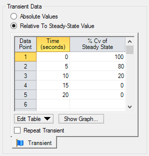
It is important to note that the loss model chosen for your valve will dictate the available transient behavior when using AFT impulse 5. For instance, if you input a Cv value in the Valve properties window, then the transient table will read in terms of Cv as shown below.

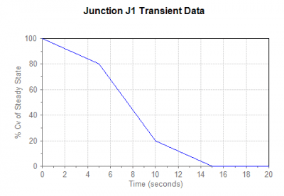
Also seen in the below image, it is possible to input a closure profile that is not entirely linear. This can be used to model the most of complex profiles. But it is important to understand that the point’s in-between input values will be linearly interpolated. With that being said, it is imperative to make sure that there is a high enough resolution in regards to your closure profile when modeling complex behaviors.

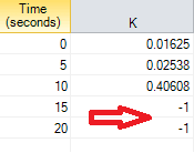
The “In’s and Out’s” of specifying a valve transient are discussed in an AFT video tutorial. There are some transient behaviors to be aware of now, however. For flow coefficients, zero indicates a fully closed valve. Inversely, the higher the value, the greater the capacity for flow, and thus the less resistance present. For a valve using the K factor, infinite resistances means that the valve is closed. To input this in AFT Impulse 5, you will need to use “-1” instead of infinity. Because the flow factor is so similar to the flow coefficient, you can apply the same principles as Cv values.

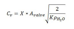
It is possible to convert analytically between loss models using the definitions above in the equation below. Note that the conversion factor will change depending on the units you are using initially!

It can be complicated to replicate a closure profile between differing loss models. If a Cv closure sets a valve to an open percentage of 80% from a steady stave Cv = 1,000, the new Cv value used will be 800. This is not the same as using 80% of the K factor equivalent, 0.01625. In fact the percent of steady state value for the K factor to equal a Cv of 800 would be 156%. As such, using a linear profile for a Cv valve will not yield the same behavior as a linearly closing K factor valve.

Clearly when trying to input a closure profile it is very important to keep track of the loss model chosen and understand the relationship to pressure drop for the modeled valve! Be sure to check out for the valve closures video tutorial for tips on inputting a closure profile using AFT Impulse!