


AFT Blog
Welcome to the Applied Flow Technology Blog where you will find the latest news and training on how to use AFT Fathom, AFT Arrow, AFT Impulse, AFT xStream and other AFT software products.
7 minutes reading time
(1417 words)
Non-Newtonian Fluids - How to Model the Soap, Silly-Putty, or Shampoo in Your Pipe Network
Non-Newtonian fluids are something almost every elementary school student is familiar with. Mixing cornstarch and water to create a liquid that acts as a solid is an experiment which has captured the attention of children (and adults) for generations. The Discovery Channel show Mythbusters even showed Adam Savage walking across a tub of cornstarch and water.
For young students, knowing that the liquid acts like a solid when impacted is enough to satisfy their curiosity. For engineers though, it is important to understand the science and math behind non-Newtonian fluids in order to accurately model how they will behave in a pipe network.
As we discuss non-Newtonian fluids here, we will cover three major topics: what it means for a fluid to be non-Newtonian, how non-Newtonian fluids are modeled mathematically, and how AFT software models non-Newtonian fluids.
What is a Non-Newtonian Fluid?
A non-Newtonian fluid is a fluid whose viscosity is dependent on the instantaneous shear rate of the fluid. If viscosity is defined as the resistance a fluid has to deformation, then a non-Newtonian fluid is one whose resistance to deformation depends on the speed at which that deformation is occurring. A Newtonian fluid on the other hand, is a fluid where the viscosity is constant across any rate of deformation.
Types of non-Newtonian fluids include dilatants, pseudoplastics, Bingham plastics, and Bingham pseudoplastics. Non-Newtonian fluids even include those whose viscosity depends on the shear rate history of the fluid, meaning the viscosity changes as the fluid is deformed at a constant rate. Time-dependent viscosity is a fascinating field of study, though as it falls outside the scope of most engineering applications, we will ignore this subset of fluid types.
A figure many readers may be familiar with is shown in Figure 1 below, plotting shear stress (τ) against shear rate (γ) for the types of non-Newtonian fluids mentioned above. For each type of fluid, the plotted curve describes the force required to shear the fluid at a given rate.

Figure 1: Plot of shear stress vs shear rate for a Newtonian fluid and four non-Newtonian fluids.
Figure 1, above, shows the general behavior of each type of non-Newtonian fluid. A Dilatant fluid begins to shear immediately, then thickens as it shears at a higher rate. A Pseudoplastic fluid starts shearing as soon as any force is applied to it, then decreases in viscosity as it shears at a higher rate. Oobleck (the mixture of cornstarch and water) and paint are examples of Dilatant and Pseudoplastic fluids, respectively.
The Bingham Plastic and Bingham Pseudoplastic fluids both have a yield stress associated with them. Toothpaste and peanut butter are examples of fluids with a yield stress. Small amounts of force applied to the fluid will not deform the fluid, but once enough force is applied, the fluid can deform and flow like any fluid without a yield stress. A Bingham Pseudoplastic fluid has a yield stress, but also decreases in viscosity as it shears at higher rates.
How to Model Non-Newtonian Fluids Mathematically
Numerous models exist to capture the real behavior of non-Newtonian fluids. We will discuss the three major models: the Power Law model, the Bingham Plastic model, and the Herschel-Bulkley model. These three models are perhaps the three most commonly used, and together capture almost the entire range of non-Newtonian behavior.
The Power Law model is perhaps the most commonly used of the three, and is used to capture the behavior of Dilatant and Pseudoplastic fluids. This model is sometimes referred to as the Ostwald-de Waele relationship model. Non-Newtonian fluids which can be described by this model are often called Power Law fluids. The Power Law model relates the shear stress applied to a fluid with the shear rate of the fluid using Equation 1, below. Similarly, the model relates the apparent viscosity of the fluid with the shear rate of the fluid using Equation 2. In Equation 2, η is used to denote apparent viscosity.
In Equations 1 and 2, K and n are the Power Law constants, and are empirically determined for an individual fluid. K has units of viscosity (centipoise is a commonly used unit), while n is dimensionless. A value of n larger than 1 represents a dilatant fluid, where η increases with γ, while a value of n smaller than 1 represents a pseudoplastic fluid. A value of n equal to 1 simplifies the Power Law model to a Newtonian fluid, with K representing the fluid's viscosity.
The Bingham Plastic model is another commonly used model, and describes the behavior of – you guessed it – Bingham Plastic fluids. Equation 3 below shows how the Bingham plastic model relates shear stress and shear rate using a piecewise function, while Equation 4 shows how the model relates apparent viscosity and shear rate.
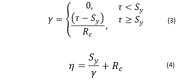
The Bingham Plastic model also has two empirical constants. Here, we've written those constants as Sy and RC, representing the yield stress and coefficient of rigidity for the fluid. The fluid yield stress can also be written as τy, τB, or τ0. Similarly, the fluid coefficient of rigidity may be written as µ∞ or ηB. Both parameters have units of viscosity. A value of Sy of 0 simplifies the model to a Newtonian fluid, with RC representing the fluid's viscosity.
Finally, the Herschel-Bulkley model is used to model a Bingham Pseudoplastic fluid, where the fluid has a yield stress and a non-linear relationship between shear stress and shear rate. To capture both behaviors, this model has three empirical parameters: τ0, the yield stress, plus K and n, as used in the Power Law model. Equations 5 and 6 below relate shear stress to shear rate and apparent viscosity to shear rate, respectively.

In the Herschel-Bulkely model, a value of n equal to 1 would reduce the model to the Bingham Plastic model, while a value of τ0 of 0 would reduce the model to the Power Law model.
How AFT Software Models non-Newtonian Fluids
AFT software offers 5 different non-Newtonian fluid models: two pulp and paper stock models (Duffy Method and Brecht & Heller Method), the Power Law model, the Bingham Plastic model, and a Homogeneous Scale-up model meant to accept empirical data from fluids that may not fit other models. Here, we'll focus just on the Power Law and Bingham Plastic models.
Fathom and Impulse implement models taken from Darby's Chemical Engineering Fluid Mechanics textbook to model Power Law and Bingham Plastic fluids. These models are described in more detail in the original text or in the topics on non-Newtonian fluids in the Help file for each application.
Darby's models create an analogous Reynolds number for each fluid, and use that in correlations to determine the Fanning friction factor in each pipe. With the Fanning friction factor, Fathom and Impulse are able to use their standard solution methods to determine pressures and flow rates in the system. Again, more details of how these models are implemented can be found in the Help file for each application.
These models allow Fathom and Impulse to capture the actual effective fluid viscosity in each pipe in the system, including the yield stress of a Bingham Plastic fluid. Table 1 below, shows some results from the Non-Newtonian Phosphates Pumping example model in Fathom with a shear thinning fluid.
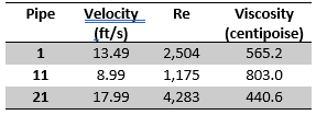
Table 2: Velocity, Re, and Average Viscosity for a shear thinning fluid at different velocities.
In Table 1, we can see the pseudoplastic nature of the fluid in action: as the fluid velocity – and the fluid shear rate – increases, the viscosity of the fluid decreases.
Non-Newtonian fluids are a vastly complex topic. This blog only begins to scratch the surface of what non-Newtonian fluids are and how they behave. Further information about how AFT software models their behavior can be found in our Help file, or by reaching out to our support engineers at This email address is being protected from spambots. You need JavaScript enabled to view it..
Comments