AFT Blog
Modeling the Stack Effect in AFT Arrow
AFT Arrow solves all of the fundamental controlling equations governing gas dynamics. For more information about which fundamental thermodynamic equations are solved in AFT Arrow, here is an excellent article that discusses gas flow calculations in detail.
The "stack effect" is simply one aspect of these equations, and is accounted for by the user input and boundary conditions. Ultimately, flow is driven by pressure difference. The higher you raise a chimney, the lower the atmospheric density and pressure at the discharge.
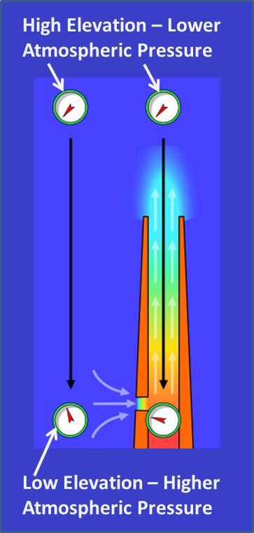
In order to accurately model the "stack effect", the system boundary conditions must be modeled accurately. As the discharge elevation of a chimney increases, then the system boundary pressure condition at the top of the stack must decrease accordingly. The figure below illustrates the stack effect quite well in regards to what the pressures would look like at different elevations.

As you can see in the above image, there are two columns of air. The left column of air is at atmospheric conditions. The lower elevation at the bottom of the air column has a higher pressure than the higher elevation point of the air column.
The pressure at the top of the chimney stack is the same as the atmosperic pressure at the same high elevation point in the column of air.
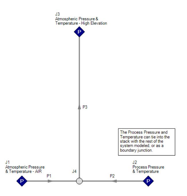
This pressure difference of the atmospheric air column needs to be accounted for in the model in order to accurately model the stack effect. The best way to model the stack effect in AFT Arrow would be with using three assigned pressure junctions.
The below image illustrates an example of how one might model the stack effect in AFT Arrow. The assigned pressure junction on the left would be specified with the ambient atmospheric pressure conditions (pressure, temperature, and elevation). The connecting pipe can be short and perhaps frictionless or hydraulically smooth to minimize the pressure drop. The assigned pressure junction on the right would have the pressure and temperature (and elevation) of the process at the base of the stack. Or, the rest of the process system can tie into the stack at this location.

Finally, the assigned pressure junction at the top of the stack would be specified at atmospheric conditions at the higher elevation point (pressure, temperature, and elevation). At this point, the atmospheric pressure will be lower than the atmospheric pressure at the elevation of the bottom of the stack.
Fundamentally, the pressure at the top of the stack needs to be lower than the atmospheric pressure and process pressure at the bottom of the stack in order to drive the flow up the stack. By defining these boundary conditions properly, the density differences will be accounted for properly for the stack effect.


Comments 5
good, it's easy to unstand this normal phenomenon by this instruction.
Great. When defining the high and low boundary atmospheric pressures to illicit the stack effects, do you tend to select these pressures as stagnation or static pressures?
Hi Ryan,
Regarding the atmospheric conditions, you will probably want to use stagnation pressures. That being said, when considering an "infinite" medium of ambient conditions where there is essentially the absence of fluid motion, then the static and stagnation conditions will typically be equal. Here is an excellent video that will help illustrate when it is appropriate to use static or stagnation conditions, https://www.aft.com/static-vs-stagnation-pressure.
Hope this helps!
Hi Ben,
Is there any chance AFT posting a worked example of this topic somewhere (I couldn't see an example in the files that came with Arrow). I've tried implementing the stack effect with the method shown, and some variations, but the results don't quite match the stack effect formula Q = C.A.(2.g.h.(Ti-To)/Ti)^0.5. I don't expect the equation and Arrow to match exactly, but I do need something to check my Arrow model against.
Thanks,
Grae.
Hi Grae,
We don't have any worked examples for the stack effect at this time. However, modeling the stack would be fairly straight-forward as long as you define the inputs for boundary pressures and elevations correctly. You would have to be able to determine would your local atmospheric pressure would be at the high elevation point at the top of the stack. Keep in mind that AFT Arrow is solving fundamental thermodynamic equations, not simplified compressible flow or simplified gas flow correlations, including the stack effect equation. Therefore, your results in AFT Arrow would be more accurate in that case. Another thing I want to point out is that the stack effect equation for Q is a volumetric flow rate. In compressible flow, the volumetric flow rate will change as pressures and temperatures change. It is not constant like in incompressible flow. Therefore, this is important to be mindful of when using a correlation compared to fundamental thermodynamics.
If you email me directly at [email protected], I can put together a quick model for you that you can use for future reference.