


AFT Blog
Welcome to the Applied Flow Technology Blog where you will find the latest news and training on how to use AFT Fathom, AFT Arrow, AFT Impulse, AFT xStream and other AFT software products.
3 minutes reading time
(587 words)
Making Sense of xT – Valve Loss in Compressible Flow
Almost every piping system has valves, and an accurate solution requires accurate valve losses. For incompressible systems, this is relatively straightforward. What happens when we introduce the complexities of compressible flow?
Valve Sizing Equation in Incompressible Flow
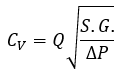
In liquid flow - like that calculated by AFT Fathom or AFT Impulse - valves are most commonly represented by the flow coefficient CV. CV is often presented as unitless but does in fact have units. It represents the gallons per minute of water that will flow through a given valve when there is one psi of pressure drop across the valve.
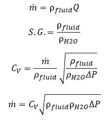
It is helpful to modify this equation to be in terms of mass flow.
Defining a conversion factor N

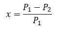
And the pressure drop ratio x
The equation becomes
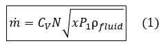
Where mass flow is in pounds mass per hour. Equation (1) is valid only for incompressible flow.
Graphically, this looks something like below.
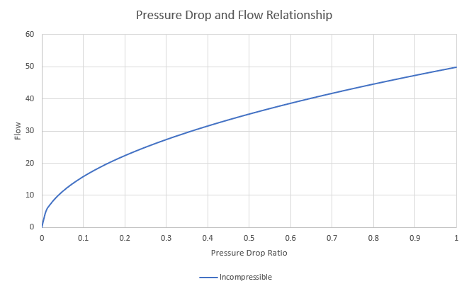
Figure 1: An example of the incompressible sizing equation being used on gas flow
Compressible Flow
There are two significant effects we need to account for if we want a similar equation for compressible flow.
- Density changes through the valve
- The flow can choke in the valve – the velocity cannot exceed Mach 1 without a converging-diverging nozzle
In gas service, CV is still the most readily available value for describing valve loss. However, as an incompressible parameter, CV alone is not sufficient to capture the above behavior.
We can account for these effects with the introduction of one more parameter – xT. xT is the terminal pressure drop ratio. This represents the smallest pressure drop ratio x for which the valve is choked. Increasing x beyond this limit does not increase flow.
Where do you get xT? Just like CV, it must be determined by testing the valve.
We can represent this in our previous equation by simply stating that, for the purposes of the sizing equation, is limited to .
Graphically:
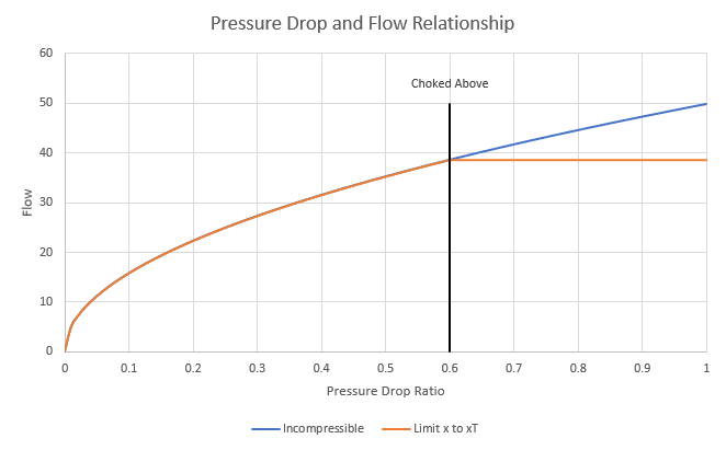
Figure 2: Including xT to represent choking
Note that this is an example only! The value of xT for a real valve depends on the particular valve design.
Applying only this change limits the flow to the sonically choked flowrate but does not address the compressibility of the gas. Without correction, this also introduces a discontinuity in the flow at x = xT.
The solution is to add an expansion coefficient Y to the sizing equation.
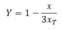
This coefficient will vary between 1 at no flow and 2/3 at choked flow. Because density is changing, we must also modify the sizing equation to include inlet density instead of an unchanging density.
Graphically:
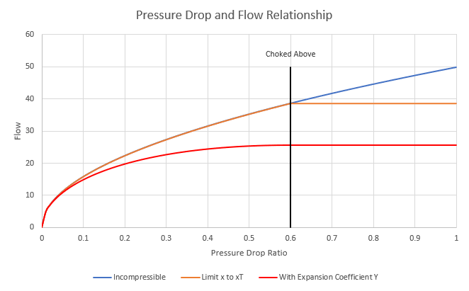
Figure 3: Accounting for the changes in density with the expansion coefficient Y
There is more loss compared to the incompressible equation as the pressure drop is higher, and a correspondingly lower flow.
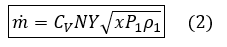
Note that Equation 2 above follows the form described by ANSI/ISA 75.01.01. The full standard considers additional effects due to gasses other than air, fittings, and changes in pipe diameters. The full version is implemented in AFT Arrow.
Comments