AFT Blog
Start your engines! Modeling an Inertial Pump Startup
There are many (six!) ways to define a pump transient event in AFT Impulse. This gives you great flexibility in creating a model that behaves the way you want it to.
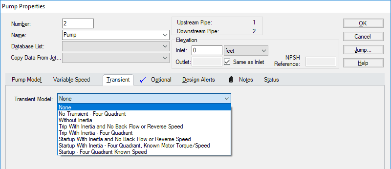
One thing true for all pumps is that they must be started at least once. Pump startups often cause significant transient effects on the system so you may wish to model this with AFT Impulse. Even narrowing your pump transient down to a startup, there are still four models left to choose from:
- Without Inertia
- Startup With Inertia and No Back Flow or Reverse Speed
- Startup With Inertia - Four Quadrant, Known Motor Torque/Speed
- Startup - Four Quadrant Known Speed
Models 1 and 4 do not consider inertial effects and require a speed vs time startup profile – but what if you do not know this speed? What if you simply want to “turn on” a pump and see what happens?
You can do this with AFT Impulse’s Startup with Inertia models! These models calculate and characterize the behavior of the pump as though the driver has been immediately switched on, accounting for the inertial resistance of the fluid, motor, and impeller. As these are more complex models, more input is required to define them.
Models 3 and 4 require additional data beyond a typical pump curve. This data, known as Four Quadrant data, is necessary to fully characterize a pump for all the flow situations it may encounter. Pumps normally operate with forward speed and forward flow. In transient situations, however, you may have any combination of forward or reverse speed and flow.
If Four Quadrant data is not available and cannot be reasonably estimated, model 2 can be used which explicitly disallows back flow and reverse speed. This could be a reasonable assumption for pumps with a built-in check valve, as an example.
Models 2 and 3 are very similar. The Four Quadrant model includes the possibility of reverse flow or speed - if this does not occur the models represent the same situation and behave nearly identically.
For simplicity, the remainder of this article will be focused on the Startup With Inertia and No Back Flow or Reverse Speed model.
To demonstrate, a simple AFT Impulse model was created:

There are several parameters that must be entered to define the startup event:
- Pump Model Tab
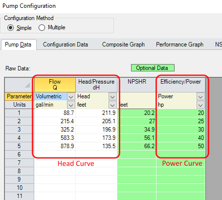
- Pump Head and Power Curves
- Transient Tab
- Start Event
- Inertial Data
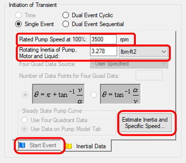
- Rated Pump Speed at 100%
- Rotating Inertia of Pump, Motor and Liquid
- Transient Data
- Optional Tab
- Special Condition
Pump Head and Power Curves must be entered on the Pump Model tab. Note that this must be power data for this model and not efficiency data.
Start Event is used to define when the event begins. This value defaults to starting the event at time zero. You can read more about how to do this here: When to Begin? Time and Events in Transient Studies.
The information necessary to determine how the pump will respond to an applied torque is defined in the Inertial Data tab: Rated Pump Speed at 100% and Rotating Inertia of Pump, Motor and Liquid. The rotating inertia field is generally not as easy to find as the rated speed. As the total rotational inertia of the system depends on the pump, liquid, and driver geometry - all of which could vary - this is not data that manufacturers would usually supply.
Fortunately, AFT Impulse provides a means for estimating the rotational inertia of the pump system. This tool requires information about operating conditions of the pump at the Best Efficiency Point (BEP). If the pump and power curves have already been defined, this data can be filled in automatically. These formulae for rotational inertia are based on linear regression analyses of pump operating points from many pumps and manufacturers – if you have a highly unusual pump it may be wise to check the inertial estimate. Estimating Pump Inertia, Specific Speed, and Four Quadrant Data within AFT Impulse 5 explains this tool in more detail.
With the rated speed and rotational inertia, the response of the system to a driving force has been defined. This driving force is entered in the Transient Data section as a Torque vs Speed curve.
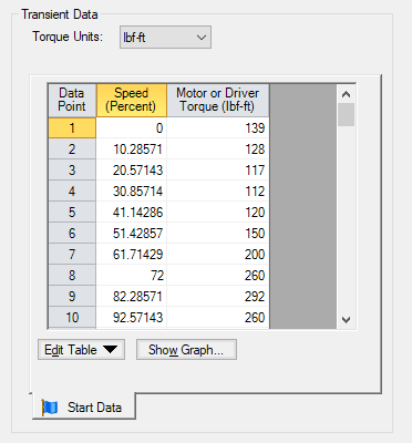
As this is a hydraulic model, it is easy to assume that the torque needed by the software is the pump torque curve – after all, this is a pump that we are defining! However, this curve is driver torque, not pump torque. Pump torque is approximately proportional to speed squared, whereas motor torque has a distinct profile vs speed, most commonly with NEMA Design B characteristics, as seen in Figure 6.
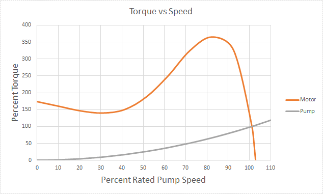
The area between the curves represents the accelerating torque of the motor and pump assembly. The coupled devices start at 0% speed and the available torque from the motor is larger than the torque resistance from the pump so the system accelerates. Acceleration continues until the operating point is met. Effects of a transient hydraulic nature such as momentum changes and pressure waves are accounted for during this process as well.
Like a Pump vs System curve, the operating point of the system after transient effects have settled out will be the intersection of pump torque and driver torque curves.
One way to determine if you are looking at driver torque is to observe the torque near zero and synchronous speed. At zero speed, driver torque is a high value referred to as Locked-Rotor Torque. At synchronous speed, the driver torque is zero.
Note that in AFT Impulse this curve is entered against Percent Rated Pump Speed whereas motor curves are often specified against Percent Synchronous Speed. To enter Torque vs Synchronous Speed data into the Transient Data table, speed values will need to be multiplied by the ratio of synchronous over rated pump speed.
Additionally, keep in mind that this is the rated speed for the pump, not the motor. Typically the two values are identical, but this is not necessarily true. In Figure 6 this intersection is past 100% Rated Pump Speed – the motor has a slightly higher rated operating speed than the pump.
Lastly, the pumps Special Condition in the Optional tab must be set to Pump Off With Flow Through.
Now that the required data has been defined, the model can be run. Below is the observed behavior of the system with the definitions given above.
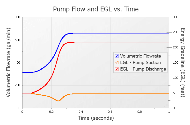
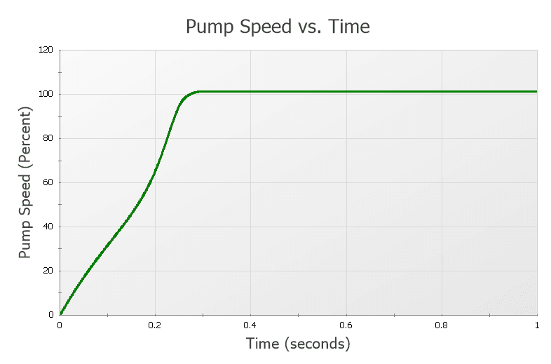
This pump starts quite quickly which significantly drops the head available at the suction – this could be the cause of serious issues including cavitation in some systems! The model will help the engineer avoid these potentialities by properly sizing the pump, or if necessary adding additional system controls to slow down its acceleration.
With a defined rotational inertia, rated speed, motor torque curve, and the pump head and power vs flow curves, AFT Impulse 6 can capture the effects of starting a motor in a hydraulic system. Now you will truly be able to get your hydraulic model started!



Comments