AFT Blog
Combining Pipes in AFT Impulse to Decrease Model Run Times: How Resistance Curves Are Merged into Pipes to Increase Pipe Section Length
They say that time is of the essence, and as engineers, that couldn’t ring truer! AFT pipe flow software is there to help engineers save time by more safely, efficiently, and rapidly designing and analyzing their piping systems.
AFT Impulse, Applied Flow Technology’s waterhammer tool, helps engineers analyze transient incompressible flow behavior that can cause potentially detrimental pressure surges. It uses the Method of Characteristics, which requires the pipes to be sectioned using a Characteristic Grid. In this Characteristic Grid, all of the pipes are broken into an integer number of section lengths, and pressure waves are assumed to propagate through each section in one timestep.
The model run time is directly affected by the number of computations needed. This number depends on the total number of time steps and the total number of sections. These parameters are related using Equation 1.
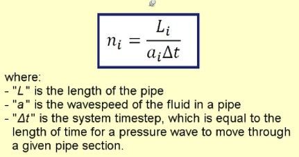
Because the number of sections greatly affects the model run time, it is of utmost importance to reduce the number of sections by making the section length as large as possible. AFT Impulse offers the ability to automatically combine pipes in order to increase the minimum section length by combining adjacent pipes with the same diameter. In this case, any pressure loss contributed by a junction connecting the two pipes will be added into the resulting pipe as a K factor. If the junction pressure loss is modeled using a component with a resistance curve, AFT Impulse will still give the user the option to combine pipes and calculate a K factor to represent the loss associated with the general component. This begs the question: How does AFT Impulse calculate a single K factor to represent a resistance curve?
The answer to this is very straightforward, and follows the process as shown below:
- AFT Impulse assumes a velocity of 5 ft/sec to determine a mass flow rate.
- A dP using this mass flow rate is then determined from the resistance curve.
- A K factor using this dP is then calculated
- If a design factor was added to the component, this value is added onto the resulting K factor
Let’s look at a model that shows this in action. See the model in Figure 1:
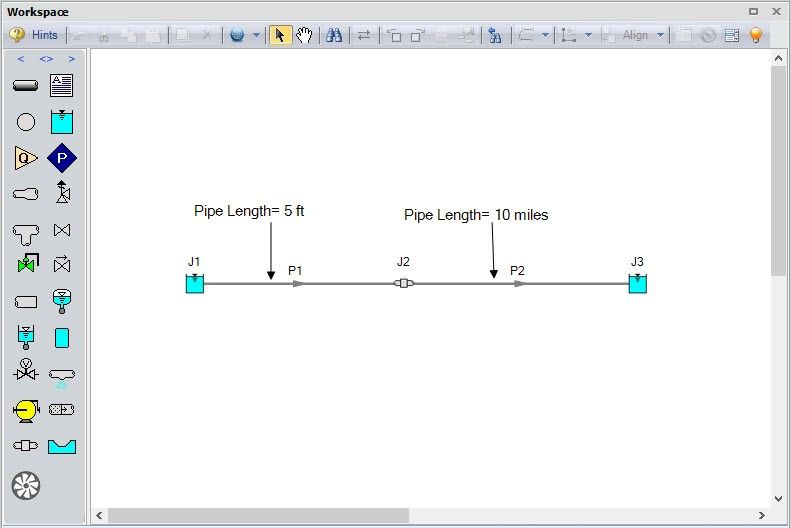
In this very simple model, the predicted run time is over 30 minutes (with a simulation duration of 200 seconds) because of the drastically different pipe lengths and the resulting large number of required sections. Assuming that there is one section in Pipe P1, there are 10,560 sections in P2 because P2 must be split up into 5 foot sections.
In order to cut the run time down, any adjacent pipes with the same pipe diameter that could be combined are displayed on the Section Pipes window (see Figure 2).
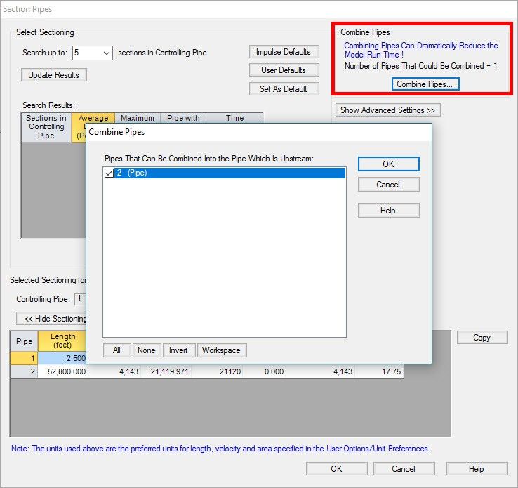
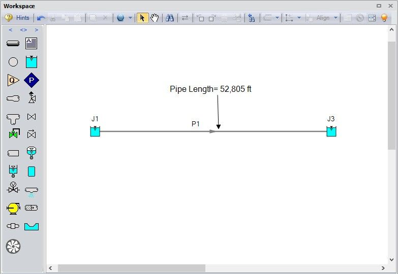
In this figure, AFT Impulse gives us the option to combine pipes P1 and P2 by calculating a K factor for the general component J2 to reduce to the run time from 30 minutes to down to less than a second. Hitting OK on the Combine Pipes window combines the pipes automatically (see Figure 3) and calculates a K factor for the resistance curve.
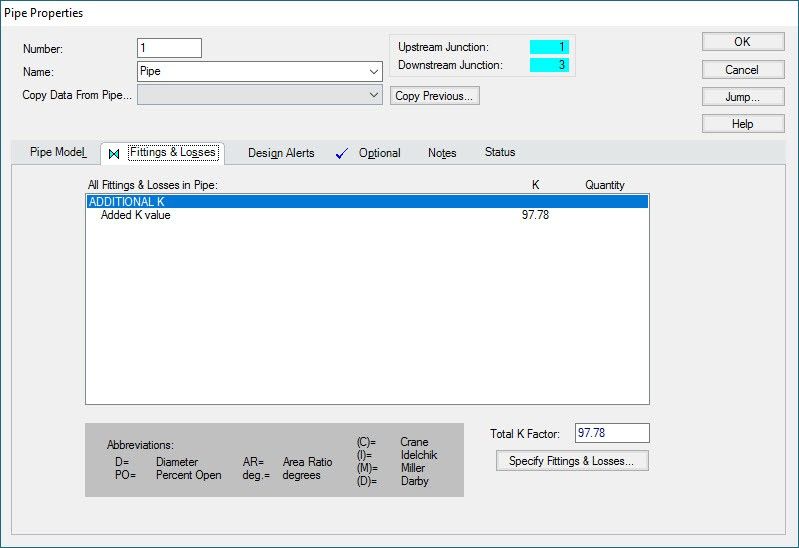
The general component is added to the Fittings and Losses tab in Pipe P1 as an additional K factor, as shown in Figure 4.
Let’s dig into how this K factor was calculated.
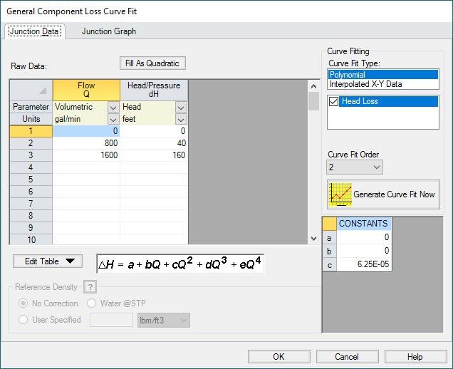
First, we assume a velocity of 5 ft/s, and calculate the mass flow rate. In this case, the mass flow rate is calculated to be 108.4 lbm/sec. AFT Impulse then takes the resistance curve of the general component (shown in Figure 5) and calculates what the resulting dP would be at this mass flow rate. For this model, the dP is determined to be 16.46 psid (this equates to a dH of 37.99 feet).
Once we have this dP, a K factor is calculated using the equation shown in Equation 2.
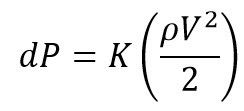
Using this equation, the K factor is calculated to be 97.78 as shown in Figure 4.
When building and analyzing an AFT Impulse model, reducing the amount of sections in the model and increasing the section lengths is frequently necessary to ensure that the model will run in a reasonable amount of time. If your model contains a component with a resistance curve with connecting pipes that have the same diameter, this curve can be converted to a K factor and added as a loss in the combined pipe. This combination of pipes can ultimately facilitate a substantially faster model run time, and as engineers, decreasing model run times equates to increased efficiency and getting your results faster!



Comments 2
Hi Erin,
This method really helps to reduce the runtime of model but in some model like the one which i have with me has few small pipes which i can't merge, and they do affect the pipe sectioning process causing a huge run time. I want to study the entire model at one time. as of now for reducing the run time i split the model in different segments. Is there any method by which i can ignore this small pipes in output and pipe sectioning process?
Regards,
Devendra
Hi Devendra,
Thank you very much for your comment, and I'm very glad that you have found this blog useful.
There is no way to ignore certain pipes in the sectioning, but what we usually recommend when engineers have models with very short pipes that cannot be combined is to perform sensitivity checks by increasing the minimum pipe length incrementally. Note that increasing the minimum pipe length is the suggested method to decrease run times because the pipe diameter has a significantly larger effect on the pressure drop than does the pipe length. The general procedure for performing these sensitivity checks is:
1) Determine the shortest pipe length and increase its length to achieve a run time you are more comfortable with. Run this model with the increased pipe length (we'll call it the "adjusted model") in the steady state, and compare the steady-state results of the adjusted model to the steady state results of the non-adjusted model. If the results are similar, there is a good chance that the change you made to the pipe length will not affect the hydraulics substantially.
2) To perform the sensitivity checks, you will need to run your unadjusted model in the transient at least once (maybe overnight to decrease its interference with your work). Once you have the results from your unadjusted model, you can compare these to your adjusted model. If the differences are negligible, you can have more confidence that changing the length of the pipes was an acceptable assumption. If you have done this for one transient and the results do not differ substantially between the adjusted and unadjusted models, you can use the adjusted model for other transients. We of course always recommend that you perform these sensitivity checks whenever possible, but following these steps can give you more confidence in pipe length adjustments you make without having to run all transients with your unadjusted model.
I hope this advice helps, and please feel free to respond to this comment below (or contact our support team at [email protected]) if you have more questions. Thanks Devendra!