


AFT Blog
Welcome to the Applied Flow Technology Blog where you will find the latest news and training on how to use AFT Fathom, AFT Arrow, AFT Impulse, AFT xStream and other AFT software products.
10 minutes reading time
(2071 words)
You Should Combine Your Pipes
One of the many powerful features in AFT Impulse is the ability to calculate transient forces during a waterhammer/surge event (See "Evaluating Dynamic Loads in Piping Systems Caused by Waterhammer" white paper). The resulting transient forces can be exported into a pipe stress analysis software. Pipe stress analysis care about what the transient forces are in a run of pipe where the piping changes direction so that proper supports can be designed. This is usually between two elbows. As piping travels all over the place in a piping network, there are lots of directional changes that need to be analyzed.
When performing a flow analysis, it is important to model the system as close to reality as possible. The more detail that is included for correct pipe diameters, length, elevation changes, fittings, and other minor losses, component losses, etc., the closer the model results will be to actual data that can be measured. However, the amount of detail that can be included in a flow model can easily become overwhelming. In AFT Impulse, including all this detail with several short pipe segments connecting fittings and components can also lead to excessively long runtimes that are unnecessary.
It is important to simplify the model while maintaining a high level of accuracy. Figure 1 below is an example of a piping system that has each of the minor losses and components explicitly modeled to visually represent direction changes.
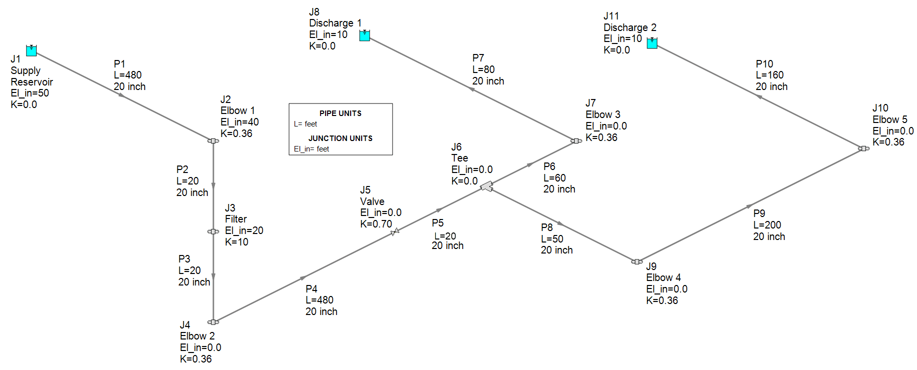
Figure 1: Complex piping system with junctions used to model point losses at the filter and elbows, elevation changes, and direction changes.
In this blog, I'm going to demonstrate that you can convert the system shown in Figure 1 into a more simplified system depicted in Figure 2, and still maintain a high level of accuracy.You can calculate all the same transient forces in the system in Figure 2 that you wound in Figure 1, even without explicitly modeling the locations of direction change with junctions.
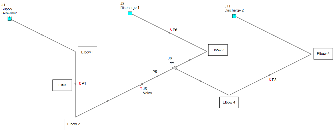
Figure 2: Combined pipe system where the losses from the filter and elbows have been lumped into the associated combined pipes. Elevation changes are included as Intermediate Pipe Elevations on the optional tab. Graphical segments maintained to represent direction changes visually.
AFT software has many capabilities that allow you to easily account for important aspects of a piping system to calculate accurate results while maintaining simplicity. One way to quickly simplify a flow model is to include the minor losses for fittings in the "Fittings & Losses" tab in the Pipe Property window. Another way to simplify a model is to model the changes in pipe elevation as Intermediate Elevations which can be done in the Optional tab of the Pipe Property window. The two blogs I linked to in this paragraph explain how to use those features.
When it comes to waterhammer modeling with AFT Impulse, it is recommended to simplify the flow model by using the Fittings & Losses as well as Intermediate Elevations features for runtime considerations. The AFT Impulse Pipe Sectioning video tutorial goes into detail about how to effectively section the pipes in your AFT Impulse model for the Method of Characteristics to avoid unnecessarily long runtimes.
A stumbling block many AFT Impulse users run into is the misconception that the piping system needs to be modeled in a detailed fashion (like in Figure 1) where junctions are used to represent losses, elevation changes, and directional changes so that transient forces can be calculated accurately for pipe stress analysis. The engineer feels stuck where they do not want to sacrifice accuracy for simplicity, but then must deal with excessively long runtimes.
The reason you CAN simplify your model in AFT Impulse (like in Figure 2), even for calculating transient forces, is because AFT Impulse assumes one-dimensional (1-D) flow. For a flow analysis, this is a valid assumption because in a flow model, the main goal is to determine flow distribution and system pressure changes. A graphical flow model greatly helps you visualize what the physical system looks like. But in order to determine pressure losses, flow rates, and transient forces, the visual direction of travel for the piping system with extra junctions and shorter pipe segments on the Workspace is not necessary for correct calculations.
Bend junctions are one of the few junction types that are not available in AFT Impulse like they are in AFT Fathom. Because Bend junctions are not components that can change over time (like a valve which can open or close), they are not included in AFT Impulse. This encourages simplicity of the model by including the losses of elbows in the "Fittings and Losses" tab of the Pipe Property window.
The explicit location of an elbow in AFT Impulse can still be modeled by using the General Component junction type with K factor and elevation data. This is what I have done in Figure 1. The way I got the K factors for the elbows was by first modeling the system in AFT Fathom using the Bend junction type accordingly. This allowed K factors to be calculated based upon the various elbow loss models available in AFT Fathom. Then when the AFT Fathom model was imported into AFT Impulse, the elbows were imported as General Components with the same K factors and elevations from AFT Fathom.
Bend junctions represent a "point loss" where the pressure is decreased at a mathematical point in a flow path based upon the K factor. In reality, a slight reflection of a pressure wave might occur during a surge event at an elbow. But this may have a minimal effect.In a one-dimensional flow model, the elbows would not cause a reflection since they are simply "point losses".To determine what is really happening through an elbow, a CFD (Computational Fluid Dynamics) analysis could be performed.
Below are four scenarios where the results comparison will validate that combining pipes will still produce very similar, if not identical results. Out of my own curiosity, I wanted to see the effect on results from using a Detailed Tee loss model to account for pressure losses across a tee compared to a Simple Tee loss model where there would be no losses. Here is an excellent blog article that goes into the associated complexities of detailed tees.
- Complex System with Simple Tee
- Complex System with Detailed Tee
- Simple Combined Pipe System with Simple Tee
- Simple Combined Pipe System with Detailed Tee
The "Complex System" represents the layout of Figure 1 where General Component junctions are used to model the elbows and filters as well as the points where the piping system changes direction. Note that the Complex System models 10 individual pipes in the entire system. The "Simple Combined Pipe System" represents the layout of Figure 2 where the minor losses from the elbows and filter have been lumped into the associated combined pipe as an additional K factor on the Pipe Fittings and Losses tab of the Pipe Property window. The elevation change is lumped into a single pipe on the Optional tab as Intermediate Pipe Elevations. The visual direction changes are identified using the Pipe Segment tool from the Arrange menu. The Pipe Segment tool allows the graphical pipe to change directions multiple times on the Workspace while remaining one physical pipe object. The Simple Combined Pipe System only has four pipes in the enter system.
The results I am going to compare for each of the scenarios include the pressure at the inlet and outlet of the valve, the pressure at the location of each elbow, and seven force sets. The results for transient pressures at the locations of the elbows can still be calculated, even when combining pipes and lumping the losses of the elbows into the pipe. Pipe sectioning creates interior pipe stations where calculations are made inside a pipe and this allows parameters to be calculated where an elbow would be, even after pipes are combined.
Figure 3 identifies the seven force sets in the piping system where the transient force differentials will be calculated. Figure 4 shows the details of how the force sets are defined in the Force Sets tab of the Transient Control window.
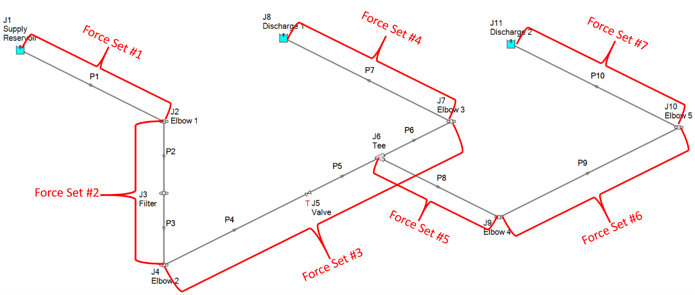
Figure 3: Seven different piping legs where the transient forces will be calculated between elbow to elbow pairs.

Figure 4: Transient Force Set details defined in the Force Sets tab of the Transient Control window
When sectioning the pipes in AFT Impulse, there is an option in the Section Pipes window to "Combine Pipes". This option will automatically combine the pipes for you. Pipes that can be combined are pipes of the same diameter that have a "static element" in between such as an elbow that does not change behavior over time (or even a valve that remains in a constant position during a transient event). When pipes are combined, all length, elevation, pipe K factors, intermediate junction losses, and the visual segmenting of the pipes will be preserved into the resulting combined pipe. Figure 5 shows where pipes can be combined during sectioning while Figure 6 highlights the pipes that can be combined from the Complex System.
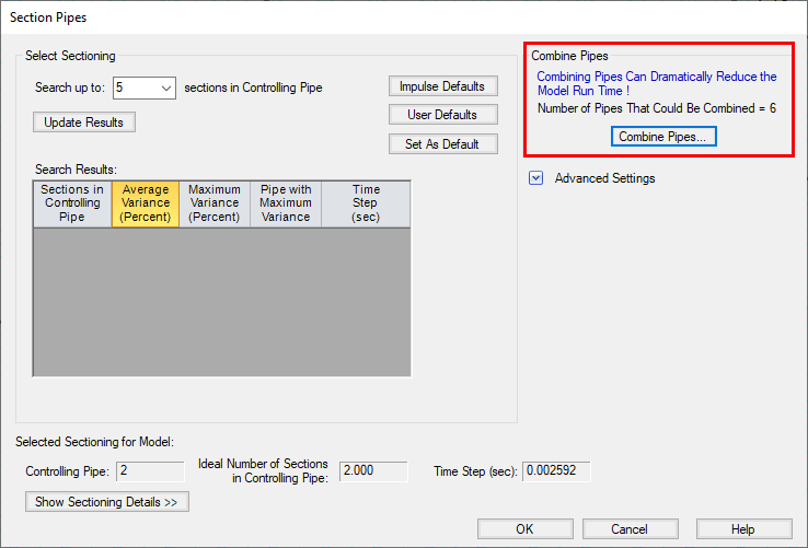
Figure 5: Combining Pipes within the Section Pipes window.
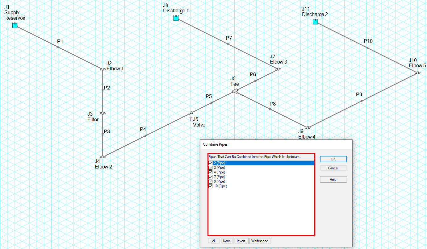
Figure 6: Six pipes in the complex system can be combined into an upstream pipe to simplify the model.
Once the pipes have been combined, the Force Sets are also preserved and updated based upon the combined pipe system as you can see in Figure 7.
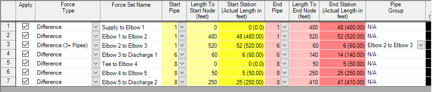
Figure 7: Force Sets tab of the Transient Control window, updated after pipes have been combined in the simplified model.
Time to compare the results of the four scenarios.
- Figures 8 and 9 compare the pressure at the inlet and outlet of the valve, respectively. As you can see, there are four data series plotted in each graph and the plotted data for each series is right on top of each other. Basically, no difference in results between complex and combined piping systems with the comparison of a simple tee and detailed tee loss model.
- Figures 10 – 14 compare the pressure at each elbow for all four scenarios. Note that in the complex system where the General Components with K factors are used to model the elbows, there is a pressure at the inlet and outlet of each junction that is calculated. When the pipes are combined as in Figure 2, there is no "inlet/outlet" pressure at the location of where the elbows are. However, the pressure at the specific pipe station of where that elbow was before it was combined can be plotted. In this blog, I'm only plotting the elbow inlet pressures to compare against the pipe station pressure for the combined pipe system.
- One thing to note in the results for pressure at the elbows is that the transient pressure is lower for the combined pipe system and higher for the complicated system. This is because when the pipes are combined and K factors are included in the pipes, the total K factor is averaged out along the pipe (i.e., the K factor is spread across each pipe station). Therefore, the pressure loss across the elbows have a smaller impact on the overall system pressure than when explicitly modeled.
- Lastly, Figures 15 – 21 compare the transient force sets for the four scenarios. As you can see, the calculated forces for each set are virtually identical! This is an excellent demonstration that the explicit modeling of junctions to represent the losses and direction changes for accurate force calculations is not necessary. The same results can be calculated for the force sets even when simplifying the model and combining the pipes.
In conclusion from this study, including the junctions to explicitly represent the location of point losses, elevation profiles, and directional changes may not be necessary and can lead to longer run times where combining pipes and simplifying the model will produce results of virtually the same accuracy. Also, accounting for pressure losses across the tee with the detailed tee loss model had very little impact.
Therefore, you should combine your pipes!
Comments 2
Seem to be missing the figures
Hello Mike - You may have some trouble seeing figures 8-21 in the PDF box located next to the content. We will look at this and determine which browsers aren't picking it up properly. Thanks for letting us know. In the meantime, here is the link for the figures: https://www.aft.com/images/easyblog_articles/536/Graph-Results-for-Combine-Pipes-Blog.pdf