


AFT Blog
Welcome to the Applied Flow Technology Blog where you will find the latest news and training on how to use AFT Fathom, AFT Arrow, AFT Impulse, AFT xStream and other AFT software products.
4 minutes reading time
(849 words)
Declutter Your Natural Gas Model
I don't have any tips for decluttering your garage or office desk, but I can offer you a tip on how to declutter your natural gas model. Perhaps it will save you some time as well in the design phase. As engineers, we like details and will enter as many as possible into our models. I've seen several AFT Arrow and xStream models with natural gas mixtures containing 8, 12, and sometimes 15 different chemical components. To add to the clutter, some of these components are measured at 0.001% of the mixture by mass. Let's see if we can come up with a simpler, de-cluttered method.
For this example, I've modeled a fictitious 24" 25-mile-long natural gas pipeline that delivers 300 MMscfd at 600 psia. There are two fluid libraries that can model chemical mixtures: Chempak, an add-on chemical library for purchase, and NIST REFPROP, which comes standard with all AFT products. For our example natural gas pipeline, we will use the NIST REFPROP library. The 4 mixtures that we will evaluate are pure methane, a methane and ethane combination, a 5-component natural gas mixture, and a 10-component natural gas mixture. The exact percentage breakdown of the mixtures can be seen in Table 1.
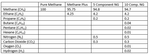
Table 1. Chemical component breakdown by mass percentage for each mixture.
Pipeline properties and model output results
In Arrow's system of equations, there are five primary properties being solved for at the junctions and along the pipes. These properties are velocity, pressure, temperature, enthalpy, and density. We can also calculate mass flow rates, Mach numbers, and stagnation properties with these properties in hand. We can then use the absolute and percent difference of these key properties between the natural gas mixtures and the pure methane to determine the significance of the chemical breakdown to the pneumatic results. The 10-component natural gas model is the most accurate because it contains the most granularity, so we will use it for our base comparison.
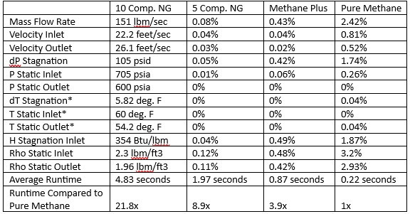
Table 2. Output results of the 10-component natural gas model properties and the percentage difference compared to the other mixtures.
(*Temperature percentage differences are calculated from degrees Rankine.)
Sure, there are a lot of numbers in the above table, but they tell a story. The first significant observation is that none of the mixtures have a percentage difference greater than 3.5%. In fact, both the 5-component natural gas model and the methane ethane mixture don't deviate more than 0.5% away from the 10-component natural gas model.
Comparing the 10-component natural gas model to pure methane, the properties that have a difference greater than 1% are mass flow rate, delta stagnation pressure, stagnation enthalpy, and both inlet and outlet densities. We have a good explanation for the difference in density results, as the mixture naturally has a higher density than pure methane. The percentage difference in mass flow rate can likewise be explained. The high percentage difference for the delta pressures is because it started with lower values to compare. 2% of 105 psi is approximately 2 psi. If this is enough to write home about, you'll need to decide. Likewise, the 0.04% for the stagnation temperature difference is about 0.2 deg. F.
How do the mixtures compare to each other?
The final significant observation is that the run time increases considerably the more components are added to the mixtures. On the high end, having a detailed mixture of 10 components has the potential to increase the run to 22 times longer than pure methane. Our example model is simple and can run in a few seconds, but we've seen models that can run for hours. Imagine waiting 4 hours between making changes to your model and receiving the results to make more changes when it could have been completed in 10 minutes, and to top it all off, you would only get a 2% increase in accuracy during the preliminary design phase.
Looking at the results outlined above, a handful of models have been sent to the AFT Support team, and my own anecdotal evidence (a.k.a. bias), it's easy for me to say, "Just use pure methane", but perhaps that's not very engineer-like or precise. Instead, let me leave you with this: when you are in the middle of your next design phase, consider for a moment using pure methane for the fluid properties of your model. Even if don't want to use pure methane, perhaps consider using a methane-ethane mixture as it will still save you computation time and keep relatively close results to the detailed composition. Once you have all your pipework, compressors, and valves in place and there are no concerning cautions or warnings to note, fine-tune your model and re-introduce your highly accurate natural gas composition. After all, you want to make sure your build will work exactly the way you designed but your time is too precious to be waiting 5, 10, or even 20 times longer than you ought for preliminary results.
Comments