To Affinity and Beyond!

Pump manufacturers often supply performance curves at a specified speed. While this is useful when the pump only runs at that rated speed, performance changes when the pump has a Variable Frequency Drive (VFD). A VFD changes the shaft speed, which, in turn, changes the performance curves. If the manufacturer only supplied a curve at a single speed, how can you know how the pump will perform when it operates at a different speed? Using the Affinity Laws, we can find the answer. This is how AFT Fathom and AFT Impulse automatically adjust pump curves to new speeds or to reach a user specified setpoint. In this blog, we will explore how the Affinity Laws apply to each parameter in a pump curve.

While one may want to apply the Affinity Laws to compressor curves, the laws are not always accurate at high compression ratios or at low Mach numbers in the compressor itself. For simplicity, the example and discussion in this blog will discuss the Affinity Laws as applied to only pump curves.

Pumps and Pump Curves

A centrifugal pump is a piece of equipment that imparts energy, in the form of head, to a flowing liquid using a spinning impeller. Two parameters that affect the head rise that a pump adds to a fluid is the speed that the impeller is spinning and the fluid flow rate. Pump manufacturers supply a curve to help engineers ensure that the expected head rise that the pump will supply is suitable for the system.

The manufacturer's curve shows the head rise that the pump will provide as a function of the flow rate through the pump. Typically, at low flow rates, pumps supply a higher head rise and low head rise at higher flow rates. Each flow rate has a unique head rise that will result from the pump. Additionally, the manufacturer's curve can include NPSHR and Efficiency or Power curves as a function of flow rate. These curves are specific to the rated speed of the pump. Sometimes the manufacturer will supply a variety of different curves for different pump speeds. But it is common for a pump curve to only display a single curve at the rated speed.

How can we know how the pump will perform when operated at a speed other than the rated speed? It is not practical to take the pump out of service then evaluate it at a variety of speeds to generate a head rise versus flow rate curve at each speed. Instead, we can use a concept called the Affinity Laws to estimate the pump performance at speeds other than the design speed. It is important to note that the Affinity Laws are only an approximation, and if pump manufacturers have performance data for different pump speeds, use those values instead.

The Affinity Laws

To use the Affinity Laws, we will use a ratio to compare the design impeller speed, N₁ to a new operating speed, N₂. N₁ and N₂ can represent either the speed in revolutions per minute (rpm) or simply the speed relative to the design speed, where 100% is the design speed.

the speed ratio, s, is equal to the rated speed, N1, divided by the new speed, N2.

Using this ratio, we can manually adjust pump curves to see what the flow rate, head rise, and power are at any speed.

We will use a pump curve and apply the Affinity Laws to it to see its performance when operated at different speeds. The data below is the data provided by the manufacturer at the pump design speed, which we will refer to as 100% speed.

Volumetric Flow Rate	Head Rise	NPSHR	Power	Efficiency
gal/min	feet	feet	hp	Percent
0	95	9	68	0
2,000	97	10	93	53
4,000	92	12	113	82
6,000	79	15	130	92
8,000	59	19	143	83
10,000	31	24	151	52
12,000	0	30	156	0

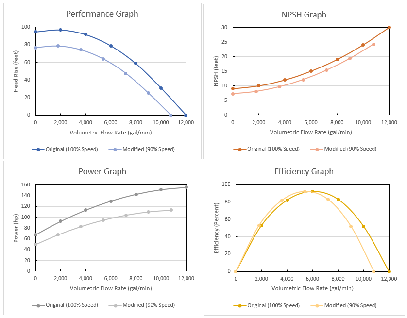
In graph form:

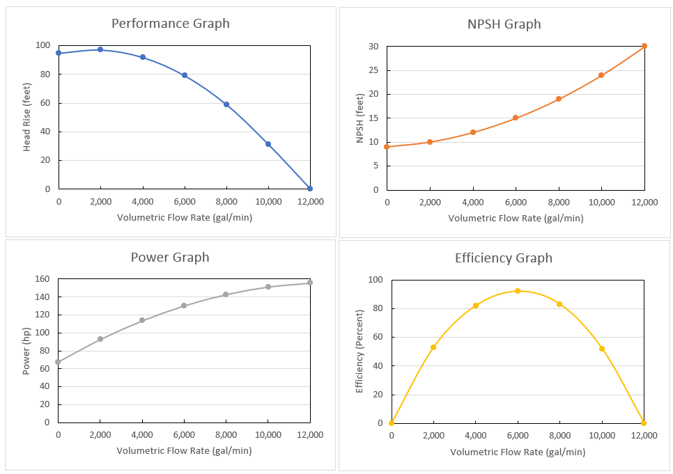
Graph form of the above table. Performance graph goes from 95 feet of head rise at zero flow to 0 feet of head rise at 12,000 gal/min of flow. NPSH graph goes from 9 feet of NPSHR at zero flow to 30 feet of NPSHR at 12,000 gal/min flow. Power graph goes from 68 hp at zero flow to 156 hp at 12,000 gal/min flow. Efficiency graph goes from zero efficiency at zero flow to a peak of about 92 at 6,000 gal/min, then back down to zero efficiency at 12,000 gal/min flow.

Note: The Pump Configuration window in AFT software only allows entry of either Power or Efficiency data, but not both, because one can back calculate efficiency from power data and vice-versa. However, to show how the Affinity Laws apply to all parameters, we are including both power and efficiency.

What happens when the pump operates at speed 90% of the rated design speed? For the sake of example, we will use the second data point: 2,000 gal/min, 97 feet head rise, 10 feet NPSHR, 93 hp, and 53% efficiency.

First, calculate s:

The speed ratio equals 100% divided by 90%, which equals 1.11.

Next, adjust the flow rate. The Affinity Laws state that the flow rate adjusts with the follow equation, where Q₁ stands for the design flow rate and Q₂ stands for the new flow rate. This law applies to both volumetric and mass flow rate.

Flow rate at the rated speed divided by the flow rate at the new speed equals s, the speed ratio.

Rearranging this equation and substituting in for s, we get

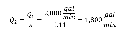
The new flow equals the rated flow divided by s, the flow ratio. This equals 2,000 gal/min divided by 1.11 which equals 1,800 gal/min.

This flow rate will be the first non-zero data point for the reduced speed pump curve. This new flow rate should make sense intuitively because a decreased pump speed will result in a lesser flow rate.

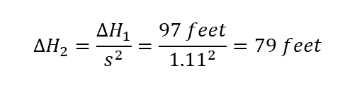
Next, adjust the head rise for the new speed. This calculated head rise will be the head rise at the adjusted flow rate calculated previously. The Affinity Laws state that the head rise adjusts with the following equation, using the same 1 and 2 conventions already established. This law applies to both head and pressure rise.

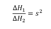
Head rise at the rated speed divided by the head rise at the new speed equals the speed ratio squared.

Note the squared s ratio. Going back to flow rate for a moment, the ratio showed that a change in pump speed results in a proportional change in flow rate. However, because of the squared speed ratio for head rise, a change in pump speed results in a squared change in head rise. When adjusting the flow rate, we saw the value decrease. The head rise for this new flow rate will decrease even more because of the squared speed ratio.

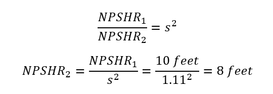
The new head ratio equals the rated head ratio divided by the squared speed ratio. This equals 97 feet divided by 1.11 squared, which equals 79 feet.

Similarly, NPSHR follows the same Affinity Law as head rise with a squared speed ratio:

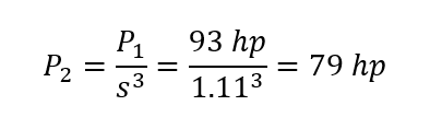
NPSHR at the rated speed divided by NPSHR at the new speed equals the speed ratio squared. Then, NPSHR at the new speed equals NPSHR at the rated speed divided by the squared speed ratio, which equals 10 feet divided by 1.11 squared, which equals 8 feet

Next, adjust power. The Affinity Laws state that power adjusts with the following equation:

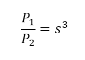
Power at the rated speed divided by power at the new speed equals the speed ratio cubed.

Note the cubed speed ratio. To repeat, the flow rate decreases proportional to the pump speed decrease. The head rise and NPSHR decrease proportional to the pump speed decrease squared. Now, the actual shaft power decreases proportional to the pump speed ratio cubed.

Power at the new speed equals power at the rated speed divided by the cubed speed ratio, this equals 93 hp divided by 1.11 cubed, which equals 79 hp

Finally, adjust efficiency. The Affinity Laws state that the efficiency adjusts with the following equation:

Efficiency at the rated speed divided by the efficiency at the new speed equals one.

The efficiency at the new pump speed is the same as the efficiency at the rated pump speed, applied to each adjusted data point.

Efficiency at the rated speed equals the efficiency at the new speed equals 53%

With all the parameters calculated for this data point, we can see that with a pump speed decrease of 10%, flow rate decreased by 10%, head rise and NPSHR decreased by 19%, power decreased by 27%, and efficiency decreased by 0%.

Repeating this process for each data point in the pump curve set, we can obtain a new pump curve for the pump running at 90% speed.

Volumetric Flow Rate	Head Rise	NPSHR	Power	Efficiency
gal/min	feet	feet	hp	Percent
0	77	7	49	0
1,800	79	8	68	53
3,600	74	10	83	82
5,400	64	12	95	92
7,200	48	15	104	83
9,000	25	19	110	52
10,800	0	24	113	0

In graph form:

Performance, NPSH, Power, and Efficiency curves with the original rated speed curves and the new modified speed. All modified curves are closer to the origin compared to the unmodified curves. The efficiency curve has the same height but has an adjusted flow rate.

We can go further and use the Affinity Laws to generate the head rise and power curves at a variety of different speeds. With a series of pump curves at various speeds, we can see what speed the pump needs to operate at to get a desired flow rate or head rise from the pump.

How AFT software applies the Affinity Laws

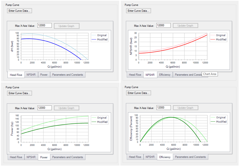
Using the Affinity Laws to calculate curves at a variety of different pump speeds may seem like time consuming work, especially if you are not sure what speed you want the pump to operate at. This is where AFT applications can save you time. All AFT applications will automatically apply the Affinity Laws to the entered pump curves. To do this, go to the Variable Speed tab of the Pump Properties window. There is a field to change the Fixed Speed of the pump. By default, this is 100% because of the assumption that the entered curve is at the rated speed. Change this to 90% and go back to the Pump Model tab. Looking at the graph preview, the properties window automatically displays a modified head or pressure rise curve, shown in dark blue in the figure. The same goes for the NPSHR, power, and efficiency graphs.

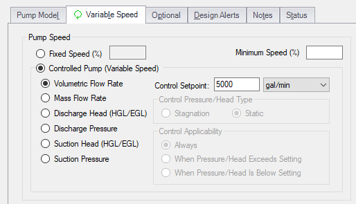
Depiction of the original and 90% speed modified curves, similar to the graph shown previously, but in the AFT software interface.

But assume the pump speed is not known. Instead, the flow rate is known and the pump speed and head or pressure rise are the desired calculated output. Going back to the Variable Speed tab, select the Controlled Pump (Variable Speed) radio button, then enter the desired flow rate. For this example, enter 5,000 gal/min then run the model.

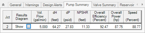
Variable Speed tab in the pump or compressor properties window. Control Setpoint of 5000 gal/min is entered.

As you can see, the solver (AFT Fathom in this case) obtained a speed of 88.77% to achieve the volumetric flow rate setpoint of 5,000 gal/min. Additionally, AFT Fathom calculates the adjusted head rise, NPSHR, efficiency, and Power using the Affinity Laws and shows these values in the output at the new pump speed.

Output showing 5,000 gal/min, 64.27 feet of head rise, 27.83 psid pressure rise, 11.33 feet NPSHR, 92.47 percent Overall Efficiency, 87.75 hp, and 88.77 percent speed

The control options offer more selections than just volumetric flow rate. Mass flow rate, discharge head, discharge pressure, suction head, and suction pressure are all available parameter options. Regardless of the parameter selected and entered, the solver operates similarly – the solver alters the pump speed, modifies the pump curve using the Affinity Laws, then checks to see if the solution meets the setpoint. If the solution does not meet the setpoint, the solver will keep repeating until it reaches the desired setpoint.

Although it may sound simple to just enter the rated pump curve and desired setpoint then let the solver do the rest, it is important to understand how the Affinity Laws work and how to apply them when obtaining hydraulic results.