Eductors, also known as jet pumps, are a clever way to pump a liquid without any rotating equipment, motors, shafts, or electricity using only the momentum from a supply fluid. However, these interesting pumps can quickly become confusing especially when trying to define them in AFT Fathom. In this blog we will explore exactly how eductors work and how to model them.
Jet Pumps / Eductors
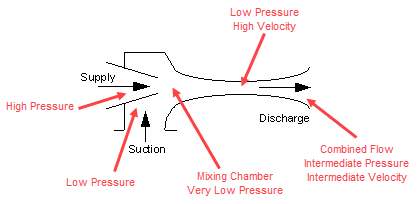
Jet pumps are devices which use a high pressure injected fluid to entrain a lower pressure fluid and induce motion, thus pumping the lower pressure fluid. It has no moving parts and utilizes fluids in motion, under controlled conditions, to provide head. Power is provided by a high-pressure stream of fluid directed through a nozzle designed to produce the highest possible velocity. The high-velocity fluid creates a very low-pressure area causing the suction fluid to flow in. An exchange of momentum occurs at this point in the mixing chamber to produce a discharge stream at an intermediate velocity. Its shape, shown in Figure 1, is to reduce the velocity gradually and convert the energy to pressure at the discharge with as little loss as possible. The high-pressure fluid is referred to as the supply (or motive) fluid, the low-pressure fluid is the suction fluid, and the combined mixture is the discharge fluid.
For a normal pump, electric energy in a motor or condensing steam in a turbine rotates a shaft connected to an impeller which transfers rotational energy into a pressure increase for a suction fluid. However, for a jet pump the energy of the supply fluid acts as the driving force to increase the pressure of the suction fluid. There will be a very large pressure drop for the supply fluid and a resulting pressure increase, yet smaller in magnitude, for the suction fluid.
The absence of any kind of rotating equipment, motors, turbines, or generators can be very attractive in some systems. This is especially true if there is a large liquid supply at high pressure that can be used as a driving force to pump a low pressure liquid.
Jet Pumps in AFT Fathom
AFT Fathom has a junction specifically for modeling jet pumps. It requires two connecting pipes: one for the suction and one for the discharge. Note that there is no pipe for the supply – this is modeled internally in the jet pump junction.
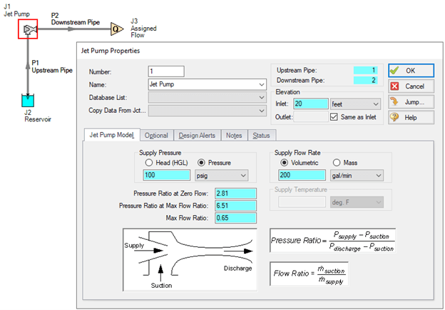
After placing the Jet Pump junction on the workspace and opening the properties window, there are several empty fields that require values before the junction is fully defined, as seen in Figure 2. Working from top to bottom, here are some definitions of the parameters needed to define a jet pump junction.
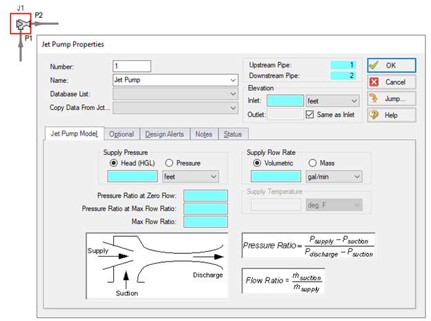
Inlet Elevation: the elevation of the jet pump relative to the reference elevation.
Supply Pressure: the pressure of the supply fluid (also referred to as the motive fluid). Note that on the workspace, there is no pipe delivering this fluid into the jet pump. The supply pressure is specified explicitly in this window and modeled internally in the junction type. This value can be specified in terms of head (HGL) or pressure.
Supply Flow Rate: either the volumetric flow rate or mass flow rate of the supply (motive) fluid. Again, there is no pipe on the workspace to deliver this fluid, it is modeled internally in the junction.
Pressure Ratio at Zero Flow: the pressure ratio when the discharge has zero flow. This is similar to how a conventional pump curve defines the pressure at zero flow where the pump curve intersects the y-axis.
Pressure Ratio at Max Flow Ratio: the pressure ratio at the maximum flow ratio. In some eductor characteristic curves, the line becomes vertical at high flow ratios. The discharge pressure to use is the highest pressure on the vertical line.
Max Flow Ratio: the maximum ratio of suction mass flow divided by supply mass flow. Of course, volumetric flow can be used here if the fluids are the same.
The latter three values are calculated using the pressure ratio equation or flow ratio equation shown in the jet pump properties window and the eductor characteristic plot in Figure 3.
Eductor Modeling Example
The following example is based on Karassik's Pump Handbook, second edition pages 4.2 through 4.9.
Suppose there is 100 gpm of suction water to be pumped up 20 feet out of reservoir at sea level using 200 gpm of supply water at 100 psig at 20 feet. A jet pump and its characteristic plot rated for 100 psig supply and 20 feet of lift is available for use. The first three required values to define the jet pump are already known: Inlet Elevation, Supply Pressure, and Supply Flow Rate. Using the pressure ratio equation, calculate the Pressure Ratio at Zero Flow.
The pressure ratio equation (shown in the jet pump properties window) is defined by Equation 1, below.
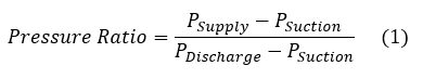
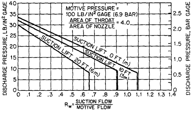
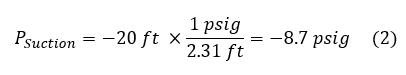
As indicated in the plot in Figure 4, the eductor is rated for 100 psig, the PSupply value. To calculate the PSuction value, convert the 20 feet of elevation gain to psig, shown in Equation 2. Since this is an elevation gain and the pressure will decrease as it goes up the pipe to the jet pump, the value is negative. The PSuction and PSupply values are the same for both pressure ratio calculations.
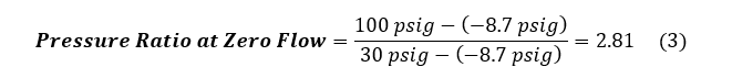
For the Pressure Ratio at Zero Flow, obtain the PDischarge value from the eductor characteristic plot, indicated in Figure 4, where the 20 foot suction lift line intersects the y-axis: 30 psig. Then use this value along with the PSuction and PSupply values to calculate the pressure ratio, shown in Equation 3, to get 2.81.
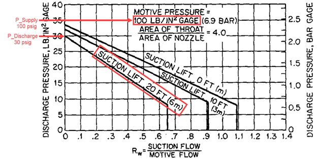
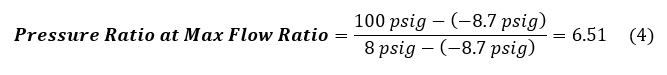
Now for the Pressure Ratio at Max Flow Ratio. Find the highest flow ratio for the 20 foot suction lift line, indicated in Figure 5, and the largest discharge pressure value at this maximum ratio is the PDischarge value: 8 psig. Using this value and the same PSupply and PSuction pressures from before, calculate the pressure ratio, calculation shown in Equation 4 below, to get 6.51. The Max Flow Ratio, also indicated in Figure 5 at the bottom, is the largest flow ratio on the suction lift line: 0.65.

Note that the pressure ratio at the maximum flow ratio is greater than the pressure ratio at zero flow: 6.51 versus 2.81. This should be expected since the discharge pressure decreases as suction flow increases at a constant supply flow, supply pressure, and suction pressure. Also note that the pressure ratios are greater than one. A pressure ratio less than one implies that the discharge pressure is greater than the supply pressure, which is not possible when the suction pressure is less than the supply pressure. And finally, note that the maximum flow ratio can be greater than one: suction flow is greater than supply flow. This is only possible at low suction lifts and low discharge pressures, but it is possible. Make sure to keep these principles in mind as a sanity check when calculating these values.
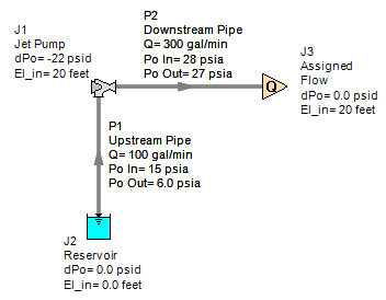
Now input these values into the Jet Pump properties window to finish defining the Jet Pump junction. The defined jet pump junction will reflect Figure 6.
Assume the pipes upstream and downstream of the jet pump are 20 feet long, 4-inch diameter, Steel - ANSI pipes. The reservoir is defined with a liquid surface elevation at 0 feet, a pipe depth of 0 feet, and a liquid surface pressure of 0 psig (atmospheric). Set the discharge of the pipe downstream of the jet pump as an Assigned Flow junction at 300 gpm (200 gpm supply flow plus 100 gpm suction flow).
Before running the model, get an idea for what the results ought to be to know if the results are correct. First calculate the flow ratio, calculated in Equation 5, and then use the characteristic plot to get the discharge pressure, indicated in Figure 7.
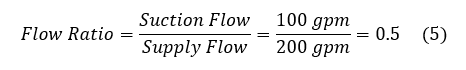
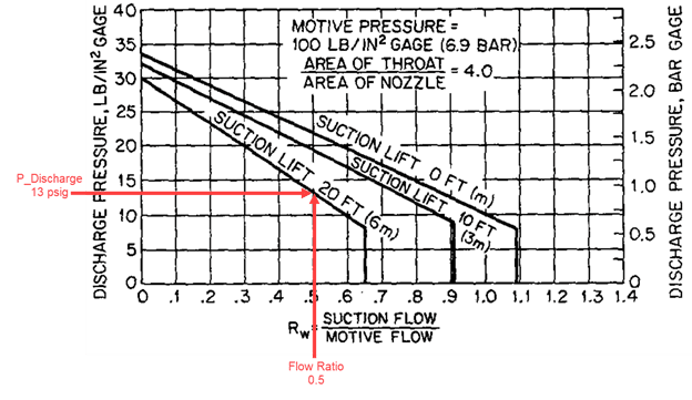
From the characteristic plot and hand calculations, a flow ratio of 0.5 should yield a discharge pressure of 13 psig (28 psia).
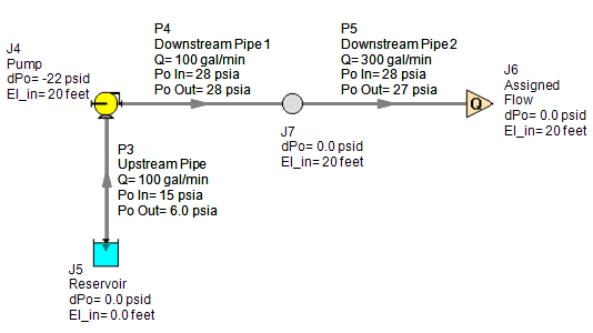
Now run the model and, as expected, the results show that 100 gpm is suctioned from the reservoir, up 20 feet into the jet pump, combines with the 200 gpm supply, and then 300 gpm discharges from the jet pump at 28 psia (13 psig). The supply fluid in the jet pump provides 22 psid of pressure rise to the suction fluid, as shown in Figure 8. It is interesting to note that the 200 gpm supply fluid drops from 100 psig to 13 psig in the jet pump in exchange for the 100 gpm suction fluid to increase from -8.7 psig to 13 psig. That is 87 psid of supply fluid pressure drop in exchange for 22 psid of pressure increase for the suction fluid, which is also half the flow rate of the supply fluid. But also remember how this jet pump provides the pressure increase with absolutely no rotational motor power or moving equipment.
In this example, the suction flowrate was known, but it may not always be known. By swapping the Assigned Flow junction with an Assigned Pressure junction or creating an entirely different system downstream of the jet pump, the suction flow can be the value that is solved for. Always double check the calculated value in AFT Fathom with the flow ratio in the eductor characteristic plot to confirm the jet pump was defined correctly.
Pump Junction Comparison
The versatility of AFT Fathom also allows a jet pump to be modeled without using the jet pump junction. The normal pump junction can be used if specified correctly. Using the values in the previous example, a pump junction will be used instead of a jet pump junction to obtain the same results.
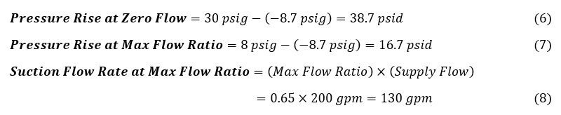
Since the jet pump characteristic plot is linear, only two points are needed to specify the curve. Using the pressure values calculated previously from the jet pump characteristic plot, calculate the pressure rise at zero flow and max flow ratio for the two points. This is simply the difference between the discharge pressure and the suction pressure, shown in Equation 6 and Equation 7. To calculate the maximum suction flow, multiply the max flow ratio, determined previously, by the supply flow, as shown in Equation 8.
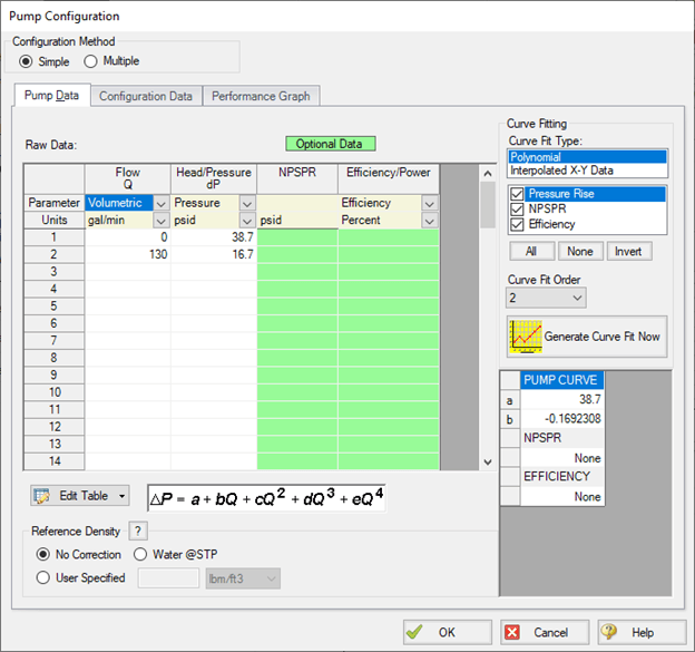
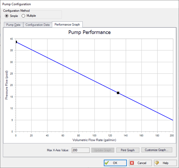
Using these values (38.7 psid at 0 gpm and 16.7 psid at 130 gpm), define the pump curve in the Pump Properties window, as shown in Figure 9. Then, with a curve fit order of 2 for a linear curve fit, generate the curve fit, shown in Figure 10.
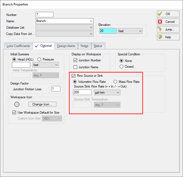
Before running the model, the 200 gpm supply flow that was modeled internally in the jet pump scenario must be included. Add a branch downstream of the pump junction with a short section of pipe connecting the pump to the branch. On the Optional tab of that branch, check the box to make the branch a Flow Source or Sink, then add the 200 gpm flow rate, as shown in Figure 11. This will add 200 gpm into the system at the branch, effectively simulating the additional 200 gpm added in the jet pump.
Run the model and the results match the jet pump scenario perfectly, as expected, shown in Figure 12. The pump provides a pressure increase of 22 psid with a discharge pressure of 28 psia (13 psig) just like the jet pump.
Not only does this method simulate a jet pump using a normal pump junction. This configuration can be used to model a jet pump if the supply flow is to be modeled externally to the jet pump junction. However, when using this method, it is absolutely critical to always double check that the flow ratio and discharge pressure matches eductor characteristic plot.
Conclusion
Jet pumps are a powerful and resourceful way to pump fluids without any motors, shafts, or moving parts. AFT Fathom provides a clear and easy way to model these systems and get the correct results. Attached are the references, models, and spreadsheets used and shown in the examples above. Feel free to take a look to see for yourself how handy the jet pump junction can be.
Now consider yourself educated on eductors!
Sources:
Karassik, Igor J. Pump Handbook. Second Edition. McGraw-Hill Book Company.