Valves are often oversimplified during modeling. Understandably, defining a valve with its range of Cv at various open percentages requires much more information than an engineer may have during the initial design phase. However, just like handbook data, heuristics, and correlations, valves too can be reasonably approximated using their common characteristics.
While valves come in all shapes and sizes, rarely will a valve have a completely unique geometry. Instead, it is easy to categorize different valves into the usual suspects: ball valves, globe valves, butterfly valves, plug valves, quick opening valves, etc. The valves in these different categories will often share common traits regarding how a valve's open percent relates to its ability to restrict flow. This relationship between a valve's Open Percent and Cv is called the valve's inherent characteristic curve. Figure 1 demonstrates a few characteristic curves for different valve types.
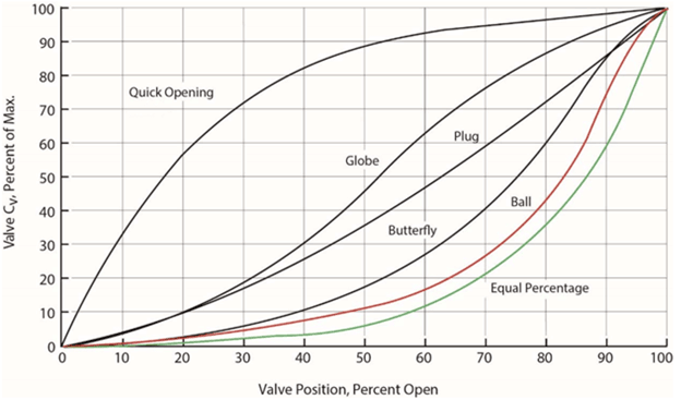
These characteristic curves are important in almost all cases, especially when evaluating a valve for a control circumstance. Even the characteristic curves of on/off valves can be valuable to consider during transient analysis.
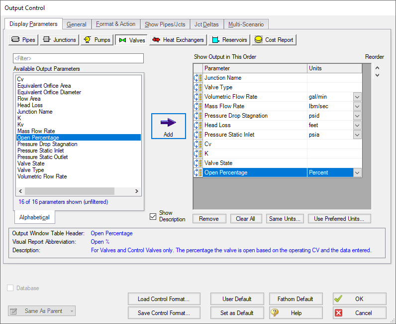
Specifying and Reporting Open Percentage
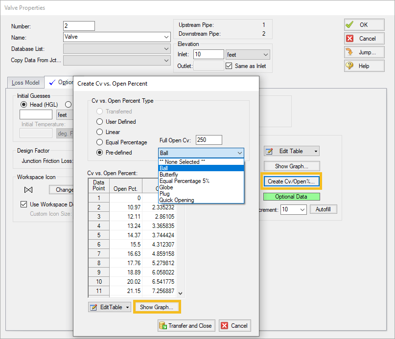
Luckily, many characteristic curves for different valve types are built into AFT software for the user's convenience. These provide a good approximation while manufacturer data has yet to be determined. In the Optional tab of the Valve Properties window, there is a button to "Create Cv/Open%...", highlighted in Figure 2. This opens a window where you can specify the Cv vs. Open Percent Type, as well as specifying the full open Cv. By knowing the full open Cv and the valve's characteristic curve, all other Open % points can be approximated. The user can also use the "Show Graph…" button to see the spread of Cv and the shape of the valve's curve.
Transient Implications
While there are some benefits to considering open percentage in steady-state, it is essential to account for valve characteristics during transient analysis as it can lead to drastically different results.
In many cases, a valve closure is simplified with a linear decrease in Cv. However, how a valve approaches a closure is almost as important as the valve's overall closure time. This is due to the valve's installed characteristic curve, or how a change in the valve's open percentage impacts flow at the system level. While entire blogs have been written about inherent and installed valve characteristics, here it is just important to understand that different valves closed over the same overall time can have drastically different results due solely to the shape of their characteristic curves.
Specifying a transient valve closure using a pre-defined characteristic curve is almost as easy as assigning the curve itself. In AFT Impulse and AFT Fathom XTS, this begins in the valve's Transient tab. Clicking Edit Table, then "Create Cv vs. Time from Open Percent…" brings you to the Cv vs. Time From Open Percent window, shown in Figure 4.
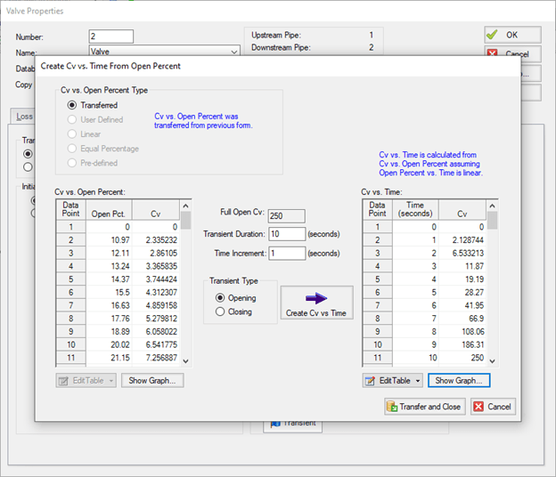
From this window, the user has several options:
- If a Cv vs. Open Percent was already defined in the Optional tab, it will automatically be transferred for use here.
- If no characteristic curve was defined, it can be fully defined here as before and saved to the Optional tab's Open Percentage Data table automatically.
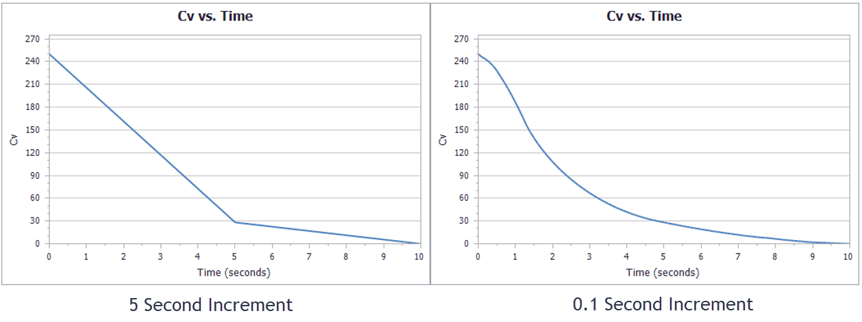
The user must also specify the overall Transient Duration time that open percent is linearly varied. The user must also define the Time Increment for the Cv vs. Time table. A smaller increment will more accurately follow the characteristic curve, while a larger increment approaches a linear Cv closure. Figure 5 below compares graphs for different time increments, generated using the Cv vs. Time "Show Graph…" button.
Finally, the valve can either be closing from fully open or opening from fully closed. Adjustments to describe other valve behaviors can always be made following the initial creation of the transient, or by manipulating the transient in excel and pasting the resulting data.
Especially during transient analysis, the valve's characteristic curve alone can drastically impact the resulting surge pressure. While this impact is also largely dependent on the system surrounding the valve, Figure 6 serves as a neat example to isolate the effects of the valve's characteristic curve. Figure 6 makes it clear that very different surge pressures are found for theoretically similar valve closures.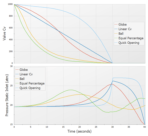
A design's safety margin may be severely impacted by considering the valve's characteristics. Luckily there are only a few extra steps to make your model a bit more precise.