This blog assumes users already know how to import engineering and cost libraries into the software. If you do not, we recommend checking out this example problem from the help file.
One of the lesser-known features of AFT products is the ability to cost out your entire system. By adding engineering and cost libraries to a model, AFT products are able to crunch the numbers and let you know how much the system will cost to build and run over its lifetime.
If you find yourself in a position where you use the same piping, pumps, valves, etc. an engineering library can help to model these junctions fast and effectively, but they can also have an associated cost library. This cost library can contain information on material, installation, and operation and maintenance costs that all AFT products will be able to reference.
Now, let's suppose an engineer had access to the aforementioned databases and wished to design an entire system utilizing the libraries at hand. He very quickly understands the system requirements and selects different pipe diameters, pump sizes, valves, etc., and lay them out in a network conducive to the necessary requirements. Feeling satisfied that the model represents a satisfactory design, it is shipped out and eventually built. This may seem like a great result, and for the most part is, but had this engineer utilized the cost libraries, he may have been able to see that with a couple of small design changes the system could function the same for a dramatically cheaper price.
Unlock the Hidden Settings
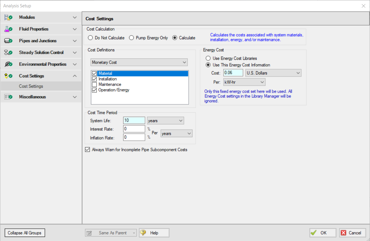
By turning on the "Cost Calculation" via the "Cost Settings" tab of the "Analysis Setup", a user can unlock the hidden settings that allow users to add a pipe or junction to the cost calculation in order to view a report of the cost of the system over its lifetime.
Taking this powerful tool into your modeling can help you to make the most efficient design choices for your system. Maybe your system can get by on running the pump at 90% speed, or maybe using smaller diameter pipes will provide sufficient flow. Regardless of how small the change may seem, these minor adjustments to the system can save a lot of money over the lifetime of the system.
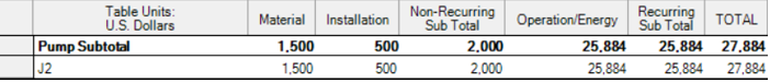
Using the example above, we can illustrate this concept. We will assume the pump is a variable speed pump and the customer wants a minimum of 400 GPM through the system. It would be very easy to model the system, see a flow rate of 439 GPM, and move on. All requirements are met (maybe even below budget), and a lifetime cost of $27,884 USD may be sufficient (Figure 2).
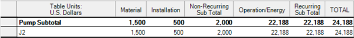
However, the majority of the cost comes from Operation and Energy. Since we have a variable-speed pump, it would be very easy to reduce the pump speed. If we set the speed to 95% (Figure 3), we would still provide 419.6 GPM, well within the design requirement, and realize a 4% drop in operation and energy costs.