Be forewarned that today I am going into full on geek mode and talk about equations for transient compressible flow. These equations are in the form of hyperbolic partial differential equations (PDEs'). If that did not scare you away yet, then you may be as much of a geek as I am! With some fancy mathematics, three PDE's can be converted into six ordinary differential equations (ODE's). From there it is a simple matter (hah!) to come up with algebraic finite difference equations. Read on!
I have been wrestling with transient flow equations for over three decades now. That is when I first started to learn about acoustic speed fluid transients in pipe systems (see What is Pogo and Why On Earth Would Anyone Want To Suppress It?). That was for liquids and it was hard enough. About six years ago I started to wrestle with compressible flow transient equations and things quickly got much more complicated.
Whether liquid or gas, the equations are hyperbolic PDE's which means they are wave equations. And wave equations lend themselves to a clever solution formulation called the Method of Characteristics (MOC). For more on this cleverness see Method of characteristics: (Why) is it so good? With the MOC one creates a fixed grid on which to solve the equations. It is this called the MOC grid.
It turns out that for transient liquid flow the equations can be made to lie nicely along the fixed MOC grid and the solution and conversion to simple algebraic equations is really not that complicated. But transient gas flow is another matter.
There have been numerous ways presented to formulate the MOC for transient compressible flow. The one in this reference (Introduction To Unsteady Thermofluid Mechanics) is particularly convenient. Not easy. Just convenient relatively speaking. Following are the three PDE's and their MOC formulation in our new AFT xStream software.

where:
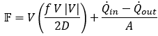
Equations 1-3 allow one to solve for three variables in space and time: P, V and ρ. Three equations. Three unknowns. Piece of cake, right?
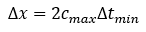
From here we need to choose a grid to attempt to integrate the above equations. For liquid flow this is quite straightforward. For gas flow it isn't. We need to figure out how far a wave can potentially travel (the distance step, Δx) in a time step, Δt. This could be very large if the flow is supersonic. We are going to limit the solution space to sonic and subsonic flows only (e.g., M <= 1).
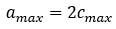
x is thus if the gas bulk fluid is traveling at sonic velocity. The maximum possible sonic velocity, cmax, will occur at the maximum gas temperature, Tmax. The maximum possible wave velocity is twice this. Why? Because an acoustic wave will travel at the fluid velocity, V, plus the sonic velocity, c. In other words, the wave speed, a, is given by:

And the maximum wave speed is given by
The maximum fluid velocity, Vmax, happens if the fluid is traveling at M = 1. In other words, when it is equal to cmax. Hence,
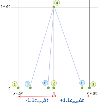
Since Δx is determined by the user's choice of pipe sectioning, then Δt is restricted by the MOC as follows:
The above equation is always stable. But it requires the shortest time step, Δtmin. Fig. 1 shows the MOC grid for this time step. Fig. 1 shows the desired computational point (location 4) using known results from points 1, 2 and 3 at the previous time step. The (R), (L) and (P) points represent the integration path for Equations 1, 2 and 3, respectively. Here (R) means the right running characteristic in the MOC, (L) is the left running one, and (P) is the particle path characteristic (not to be confused with pressure, P).

To have a faster run time (so you can get your results sooner!) you want a longer time step. Here is where you can make things solve faster and increase accuracy to boot. If you know what the maximum Mach number, M, is during your entire simulation, you can use a different grid. For example, assume you know that the maximum M is 0.1. In that case you can use the grid and time step in Fig. 2.
In AFT xStream you can use either Fig. 1 or 2, or some other time step based on the Max Mach number you select. Looking back at Figs. 1-2, something is evident to an experienced eye for the MOC – points (R), (L) and (P) do not coincide with points 1, 2 or 3. That means that to get P, V and ρ at points (R), (L) and (P) one needs to interpolate. And that introduces errors. That is why Fig. 2 is preferable to Fig. 1 for lower Mach number flows as it means less interpolation. Ideally you want points (R), (L) and (P) to be as close to points 1 and 3 as possible, and far away from point 2. Fig. 2 does this better than Fig. 1 on average.
Whichever you choose, Equations 1-3 are solved by integration over the Fig. 1 or 2 grid. This looks like below:

These three equations above are then used to solve for P, V and ρ at point 4, our desired computation point as below.

Look at those three equations. A smart 12-year-old who has taken algebra class can solve that. Three equations and three unknowns. Easy.
Well, not so fast. Boundary conditions come in at the inlet and outlet of each pipe. These are the junctions in AFT xStream. To solve a three-pipe branch or tee junction you end up with 12 equations and 12 unknowns for that junction. No typo there. Yes, really, 12.
If all we had to manage was perfect gas flow (e.g., air at low pressures) at relatively low Mach numbers (say below 0.3) things would be considerably easier. High Mach number flows for real gases like steam present some tough challenges. Even for geeks like us. That is why I titled my first blog on AFT xStream last April, Gas and Steam Transient Analysis is Freaking Hard!.